2 The Worksheet
- Worksheet layout and usage.
- Activating a worksheet.
- Adding, deleting, moving and copying a worksheet.
- Renaming and modifying a worksheet.
- Selecting with the mouse.
- The important difference between the contents and format of a cell.
- Printing and print settings.
A workbook can contain one or more worksheets. Each worksheet has a tab at the bottom of the workbook window. In the worksheet, you can enter data and formulas. This chapter covers how and where to enter data in the worksheet, and how it is displayed.
2.1 What is a Worksheet?
An overview of worksheet design and usage.
A worksheet contains rows and columns. The intersection of a row and a column is a cell. You can store data and formulas in the cell.
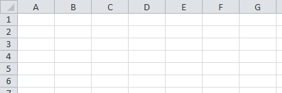
Rows are numbered 1, 2, 3, and so on, while columns are labeled A, B, C, and so on. After Z, columns are labeled AA, AB, and so on. After ZZ, the labeling continues with AAA, AAB, etc. A worksheet can contain 16,384 columns and 1,048,576 rows. This results in over 17 billion cells.
Each cell is identified by a specific row and column. The combination of the column letter and row number is called a cell address or cell reference. The first cell in the upper left corner is A1. Cell addresses can be used in formulas to refer to cell content.
A cell is selected by clicking it with the mouse. This cell becomes the active cell, and it is highlighted with a border.
A worksheet always has an active cell. You can activate a different cell by clicking it, or by using the arrow keys on the keyboard to move the active cell. When you start typing, data is entered into the active cell. Press the Enter key to complete data entry. By default, the active cell moves down one cell.
You can change this direction in File > Options > Advanced: down, up, right, and left.
The content of a cell can be:
- text
- numbers
- formulas
References to other cells are allowed in the formulas. Formulas are automatically recalculated when the content of referenced cells changes. This makes a spreadsheet very powerful.
2.2 Activating Worksheet
A workbook can contain multiple worksheets, each with its own tab at the bottom left of the window. You must activate a worksheet before you can use it. If there’s only one worksheet, it’s activated automatically. To activate a different worksheet, click its tab. The active worksheet’s tab appears with a white background.
Task 2.1 File: Consolidation.xlsx
Open the file.
Click on different worksheet tabs to select them. The selected worksheet appears, and its tab turns white.
2.3 Add a New Worksheet
Task 2.2
Open a new blank workbook.
Click on the New sheet button
 .
.
A new worksheet is added to the end of the workbook and becomes the active sheet. The new worksheet is automatically named “Sheet” followed by a number. You can rename it later (see Section 2.5).
2.4 Deleting Worksheet
It’s good practice to keep only worksheets with content and delete empty ones. You can delete any worksheet except the last one, as a workbook must contain at least one worksheet. If a worksheet contains data, or if you’ve emptied it by removing all content, Excel will ask you to confirm the deletion. Otherwise, the worksheet will be deleted immediately.
Task 2.3
- Right-click the worksheet’s tab, and then select Delete.
You’ll encounter one of two scenarios:
- The worksheet is deleted immediately. If this happens, no further action is needed.
- A dialog box will appear, asking you to confirm the deletion.
- Click Delete.
2.5 Renaming Worksheet
It’s recommended to give worksheets descriptive names instead of the default names like Sheet1, Sheet2, Sheet3, etc.
Task 2.4
Rename a worksheet using one of these methods:
- Right-click the worksheet’s tab, and then select Rename.
- Double-click the worksheet’s tab.
Type the new name, and then press Enter.
2.6 Copying Worksheet
Task 2.5
- Right-click the worksheet’s tab and select Move or Copy ...
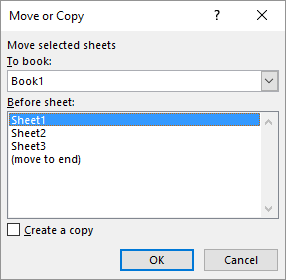
- You can perform one or more of the following actions:
- To book - This option defaults to the current workbook. Use the drop-down arrow to select a different open workbook. Selecting “new workbook” will create a new workbook.
- Before sheet - Choose the destination workbook location.
- Create a copy - Select this option to create a copy of the worksheet. If you leave it unchecked, the worksheet will be moved to the new location.
2.7 Mouse Selections
Often, you’ll want to apply a command to multiple cells at once. For example, you might want to center the text in several cells or change their font. Therefore, it’s important to become proficient at selecting multiple cells. Table 2.1 shows the most common selections.
| Desired selection | Method |
|---|---|
| single cell | Click the cell. |
| range of cells | Click the first cell in the range, and then drag it to the last cell. |
| single column | Click the column letter. |
| adjacent columns | Click the first column letter and drag it to the last column letter. |
| single row | Click the row number. |
| adjacent rows | Click the first row number and drag it to the last row number. |
| all cells in worksheet | Click the button above row 1 and to the left of column A, or use the shortcut CTRL-A |
You can also use the Shift key or the CTRL key to modify selections:
SHIFT key
The Shift key allows you to select a contiguous range.
- To select a rectangular range, click one corner cell, hold down the Shift key, and then click the diagonally opposite corner cell.
- To select adjacent columns, select the first column, hold down the Shift key, and then select the last column.
- To select adjacent rows, select the first row, hold down the Shift key, and then select the last row.
CTRL key
The Ctrl key allows you to select non-contiguous ranges. Select the first cell, range, row, or column, hold down the Ctrl key, and then select the other cells, ranges, rows, or columns.
You can only make selections when the mouse pointer is a thick plus sign
 .
.The selected area is highlighted, except for the first cell you clicked. This cell remains the active cell and has a white background.
Dragging from bottom to top or right to left is generally easier than the reverse.
Indicating areas
You can use cell addresses to specify adjacent ranges. A few examples:
A2:C7represents the rectangular range of cells from A2 to C7. Always start with the cell address of the upper-left corner, followed by a colon, and then the address of the bottom-right corner.B:Erepresents columns B through E.3:9represents rows 3 through 9.
2.8 Cell: Content and Format
A cell has content and a format. It’s crucial to understand the difference between these, as confusion often leads to errors.
Example 2.1 Content - Format
Cells A1:A10 all contain the number 40299. Therefore, these cells have the same content but appear different due to different formatting.
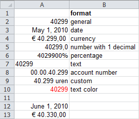
Looking at the figure it is difficult to see what the format and what the content is. Content and formatting are two different things.
Make sure that you don’t type the formatting when entering data in a cell.
For example, if you type 40.299 hours in cell A9, then it is considered as text and not as a number. And because it is a text you cannot calculate with the content.
It is possible to only enter the number and then format the cell so that it has the appearance as shown. The content of the cell is then a number with which you can make calculations.
The preferred method is to first enter the content in the cell and give the cell the desired format after that.
2.9 Printing worksheets
Things that must be done to make a good print of a worksheet.
Most worksheets with calculation models will be printed. When printing, you have many options available to customize the page layout. For example, you can choose headers and footers, margins, portrait or landscape orientation, the layout of the pages, etc.
It is recommended that before you print, you should first take a look at the print preview on the screen. From there you can then change several settings before the actual printing.
For making a print choose File > Print.
From here you can select what printer to use and what worksheets to print. By default, only the selected worksheet will be printed. But you can also choose to print multiple worksheets and even the entire workbook.
2.9.1 Print Preview
The preview shows you how the printed page will look like and gives you options to change several settings.
To judge if a print will look good, it is recommended to look at the print preview first. From there you can easily change some print settings.
Task 2.6 File: Personnel.xlsx
Open the file.
Choose File > Print.
A preview of the print and possibilities to change settings are displayed.
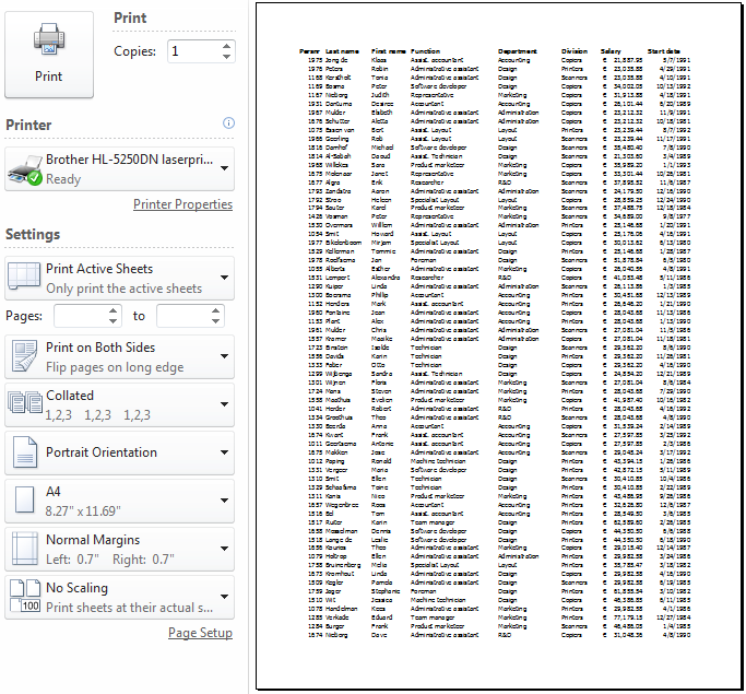
If you want to see the margins, then click on the button Show Margins at the bottom right corner of the window.
By clicking on Page Setup you get a dialog box with tabs with a lot of print options.
2.9.2 Page Setup
The Page Setup dialog box contains four tabs with various print options. The most common options are discussed here.
Page
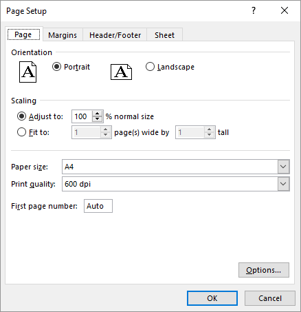
Page orientation (Portrait or Landscape) is important.
The Scaling options are very useful. Adjust to allows manual customization of the number of pages. Fit to lets Excel automatically scale the printout to a specified number of pages.
Margins
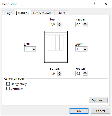
Here, you can set the top, bottom, left, and right margins, as well as the header and footer distances from the page edges. These distances should be less than the corresponding margins to avoid overlap.
Header/Footer
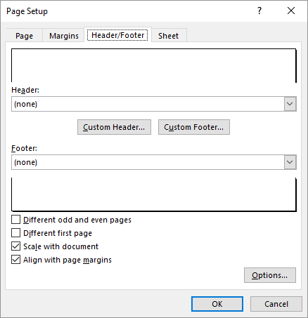
Clicking the arrow in the header and footer boxes lets you select from predefined texts or choose (none) to omit them. To create a custom header or footer, click the custom text button to open a dialog box for typing and formatting text.
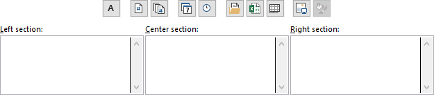
Headers and footers have left, center, and right sections. You can enter text in each section and use the available buttons to insert predefined content, such as:
- Page Number
- Number of Pages
- Date and Time
- File Path, File Name, and Sheet Name
Sheet
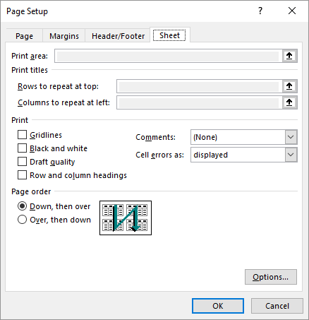
Worksheets often have titles in the first row(s) or column(s). If the worksheet spans multiple pages, you can specify how these rows and/or columns should appear on each page.
An interesting option is to print the worksheet’s gridlines.
Page Setup options are also accessible via Page Layout > group Page Setup.
2.9.3 Page Breaks
Only a limited number of rows and columns fit on a printed page. Excel automatically inserts horizontal and vertical page breaks based on factors like paper size, margins, row heights, column widths, and font. You can also manually insert, move, or delete page breaks.
Page Preview
While you can work with page breaks in Normal view, Page Break Preview is recommended. This view shows how page orientation and formatting changes affect automatic page breaks. For example, you can see how changing row height or column width alters the placement of breaks.
Choose View > Page Break Preview (group Workbook Views).
This view also displays the page order, which defaults to down, then across. You can change this order in Page Setup.
To move page breaks, drag them to a new location with the mouse.
To return to Normal view, choose View > Normal (Workbook Views group).
Inserting Page breaks
To insert page breaks manually:
- Horizontal page break: Select the row where the new page should begin.
- Vertical page break: Select the column where the new page should begin.
Then choose Page Layout > Breaks (Page Setup group) > Insert Page Break.
Deleting Page breaks
You cannot remove automatically generated page breaks. You can only remove manually inserted breaks. To do this:
- Horizontal page break: Select the row below the page break.
- Vertical page break: Select the column to the right of the page break.
Then, choose Page Layout > Breaks (Page Setup group) > Remove Page Break.
2.10 Shortcuts cell movement
| Shortcut | Active cell becomes |
|---|---|
| Arrow Up | One cell up |
| Arrow Right | One cell right |
| Arrow Down | One cell down |
| Arrow Left | One cell left |
| CTRL arrow right | Rightmost cell in the current data region, or the last cell in the row |
| CTRL arrow left | Leftmost cell in the current data region, or the first cell in the row |
| CTRL arrow up | Topmost cell in the current data region, or the first cell in the column |
| CTRL arrow down | Bottommost cell in the current data region, or the last cell in the column |
| Home | First cell in the row |
| CTRL Home | First cell in sheet (A1) |