17  Measurements

OBJECTIVES

• Explain of linear relations.
• Add a linear trendline to a scatter plot.
• Use of the SLOPE and INTERCEPT worksheet functions.

Researchers often want to know whether the value of one variable depends on another. To determine this, they conduct measurements. During these measurements, one variable is changed (independent variable), while another variable is measured (dependent variable).

These measurements produce a series of data points that can be plotted on a chart. The shape of the chart often provides an initial indication of whether a relationship exists between the variables—and if so, what kind: linear, exponential, logarithmic, etc.

A relationship between variables is represented by a mathematical function and described by an equation. If the relationship is linear, the chart will display a straight line.

When plotting measurement results, there usually isn’t a single line that fits all data points perfectly. Using statistical methods, applications like Excel can determine the best-fitting line, known as a regression line. The method used to calculate this line is called the least-squares method. The underlying statistical techniques are beyond the scope of this chapter. If you’re interested in learning more, consult additional literature.

17.1 Linear Relationship

If there is a linear relationship between two variables $x$ and $y$, it can be expressed by the equation:

$y=ax+b$

• $y$: the dependent variable
• $x$: the independent variable
• $a$: the slope (a constant)
• $b$: the intercept (a constant)

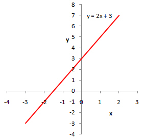
Example 17.1 $y=2x+3$

The graph of $y=2x+3$ is a straight line. The slope of the line, $a$, is 2, and the intercept (where the line crosses the y-axis), $b$, is 3.

Figure 17.1: Straight line in a linear relationship

With measurement results, you can use Excel to

• plot the data points.
• draw a trendline (best-fitting line).
• display the trendline equation.
• calculate the slope and intercept using Excel functions.

17.2 Linear Trendline

This section explains how to add a linear trendline.

At a timber factory, large numbers of similar items are produced, primarily differing in size and weight. To investigate whether production time depends on item weight, several measurements are taken. A linear relationship is assumed.

Task 17.1 File: Prodtime_Weight.xlsx

1. Open the file.

2. Select the range A2:B11, which contains the measurements.

3. Go to Insert tab> Recommended Charts (Charts group) > Scatter > OK.

4. Add a linear trendline.

You can add a trendline in the following ways:

• Click the data points in the chart, right-click, and choose Add Trendline.
• Select the chart area, click the button next to it, and choose Trendline > Linear.

5. Select the trendline and Right-click > Format Trendline.

6. In the Format Trendline pane, check Display equation on chart.

Figure 17.2: Trendline options.

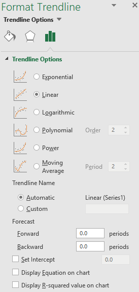
7. Make the following adjustments (see the example in Figure 17.3):

   • Add a chart title and axis titles.
   • Adjust the axes scales.
   • Remove decimal places from axis labels.
   • Set the trendline color to solid red.
   • Move the equation to a visible location.

Figure 17.3: Scatter plot of the measurements with linear trendline.

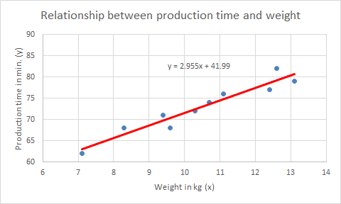
From the trendline equation, you can determine the relationship between the variables:

$Productiontime=2,955\times Weight+41,99$

Worksheet functions

You can use Excel’s statistical functions SLOPE and INTERCEPT to find the slope and y-intercept of the trendline.

8. In an empty cell, insert the SLOPE function with the following arguments:

   • Known_ys: B2:B11
   • Known_xs: A2:A11

9. In another cell, use the INTERCEPT function with the same ranges.

The slope is 2.95503212 and the intercept is 41.99036403, which correspond to the trendline equation.

17.3 Exercises

Exercise 17.1 Height and Weight (meas001)

File: Meas001.xlsx

The height and weight of several schoolchildren are shown below.

Height and weight results.

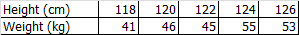
Assume a linear relationship and determine the equation where weight is a function of height.

Weight = 1.65*Height - 153.3

Exercise 17.2 Study Time and Exam Grade (meas002)

File: Meas002.xlsx

The study time and exam scores of several students are shown below.

Study time and exam scores.

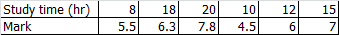
Assume a linear relationship and determine the equation where score is a function of study time.

Mark = 0.2038*Study time + 3.3637

Exercise 17.3 Shrinkage and Temperature (meas003)

File: Meas003.xlsx

A synthetic fiber manufacturer investigates whether fiber shrinkage relates to the washing temperature. Eight experiments are conducted at different temperatures. Shrinkage is expressed as a percentage of the original length.

Shrinkage percentage vs washing temperature.

1. Assume a linear relationship and determine the equation where shrinkage percentage is a function of temperature.

2. Predict the shrinkage at a temperature of 65^oC.

Shrinkage = 0.0796*Temp - 3.546

At 65°C, the predicted shrinkage is 1.6%.

Exercise 17.4 Resistance and Temperature (meas004)

File: Meas004.xlsx

The resistance of a metal block is influenced by temperature. The figure below shows resistance at various temperatures.

Resistance at various temperatures.

1. Assume a linear relationship and determine the equation where resistance is a function of temperature.

2. Predict the resistance at a temperature of 400^oC.

Resistance = 0.0786*Temp + 21.214

At 400^oC, the predicted resistance is 52.6 Ohms.