8 Array Formulas

OBJECTIVES

Introduction to arrays.
Creating array formulas.
Create frequency distribution of data with FREQUENCY function.
Dynamic arrays and associated functions.
Mathematical array functions.

An array formula is a formula that can perform multiple calculations on one or more items in an array. Array formulas used to be considered tricky because they look different from regular formulas and required a special entry method: pressing CTRL+SHIFT+ENTER instead of just ENTER. This is no longer the case in Excel 365.

In Excel 365, the behavior of array formulas has changed compared to other Excel versions. Existing formulas that produce multiple results now behave like array formulas. Several new dynamic array formulas are added to Excel 365.

Therefore, much of this chapter applies primarily to Excel 365.

8.1 What is an Array Formula

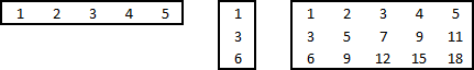
A vector is a list of numbers arranged in either a row or a column. A row of numbers is called a row vector, and a column of numbers is called a column vector. Excel uses the term “array” instead of “vector.”

In Excel, an array can be:

A row of values (a row vector or a 1-dimensional horizontal array).
A column of values (a column vector or a 1-dimensional vertical array).
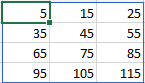
A rectangular block of rows and columns (a 2-dimensional array).

Figure 8.1 illustrates each type.

Figure 8.1: Array examples (from left to right): row vector, column vector, 2-D array.

You can create an array using constant values, as shown in the examples, by starting a cell entry with the = symbol and enclosing a row of values in curly brackets {}. The values must be separated by a specific symbol. The appropriate separator depends on the language and regional settings of your computer.

For English language systems:
- Use a comma (`,`) to separate values in a row (new column).
- Use a semicolon (`;`) to separate rows.
For Dutch language systems:
- Use a backslash (`\`) to separate values in a row (new column).
- Use a semicolon (`;`) to separate rows.

Additionally, 2-dimensional arrays must follow these rules:

List values in row order.
All rows must have the same number of columns.

Here are some examples:

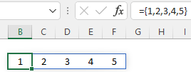
Example 8.1 Row vector

={1,2,3,4,5} returns 1 row with 5 columns.

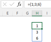
Figure 8.2: 1-dimensional horizontal array.

Example 8.2 Column vector

={1;3;6} returns 3 rows with 1 column.

Figure 8.3: 1-dimensional vertical array.

Example 8.3 2-dimensional array

={1,2,3,4,5;3,5,7,9,11;6,9,12,15,18} returns 3 rows with 5 columns.

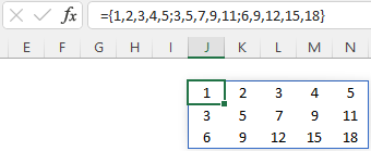
For all the above examples, only the first cell where you entered the array formula is editable. When you select any other cell within the array’s range, the content in the formula bar appears grayed out, and you cannot change its value.

8.2 Simple Array Formulas

An array formula performs calculations on arrays, and the result is also an array. When using array formulas, you need to determine in advance how many results to expect and how those results should be arranged (in a single cell, row, column, or table).

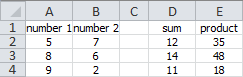
In Figure 8.5, you can see the sum and product of two numbers calculated multiple times. This can be done with simple formulas. For instance, the formula in cell D2 could be =A2+B2, and the formula in E2 could be =A2*B2. Copying these formulas down would apply the correct formulas to D3:E4.

Figure 8.5: Sum and product of two numbers using regular Excel formulas.

However, these calculations can also be performed using array formulas, which is a good practice for understanding how they work.

Task 8.1 File: Array1.xlsx

Open the file.
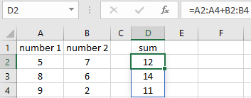
Select cell D2 and enter =A2:A4+B2:B4, then press ENTER. The results appear in cells D2:D4, with a box around them indicating an array.

Figure 8.6: Sum of two columns using an array formula.

Selecting cell addresses with the mouse is easier than typing them.
Since the addition results in a column of three numbers, Excel automatically spills the results into cells D3:D4. Ensure these cells are empty beforehand to avoid a #SPILL! error.

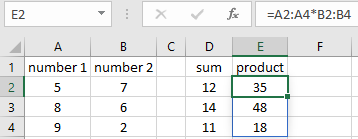
Select cell E2 and enter =A2:A4*B2:B4, then press ENTER. The results appear in cells E2:E4, with a box around them indicating an array.

Figure 8.7: Product of two columns using an array formula.

Task 8.2 Multiplying a row vector by a constant

Figure 8.8 shows a row of three numbers multiplied by 4. The result is a row of three numbers. Try this example yourself.

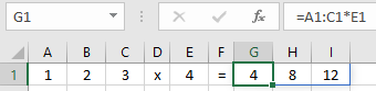
Figure 8.8: Multiplying a row vector by a constant.

Formula in G1: =A1:C1*E1

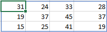
Task 8.3 Multiplying a 2-dimensional array by a column vector

Figure 8.9 shows a 4x3 array multiplied by a column of numbers. The result is a 4x3 array.

Try this example yourself. You can use the practice file Array2.xlsx.

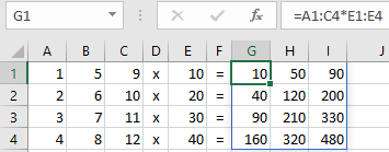
Figure 8.9: Multiplying a 2-dimensional array by a column vector.

Formula in G1: A1:C4*E1:E4

8.3 Calculating a Single Result

This section explains how to use a single array formula in situations that might otherwise require multiple formulas.

Use an array formula when you need to perform several calculations to get one result. This simplifies the worksheet by replacing multiple formulas with a single array formula.

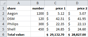
Figure 8.10 shows a stock portfolio with prices. To calculate the total value of the shares at a given price, you would typically calculate the value for each stock and then sum those values. An array formula can perform this calculation without intermediate steps.

Task 8.4 File: Array3.xlsx

Open the file.
Select cell C6 and enter the formula =SUM(B2:B5*C2:C5).
Repeat for cell D6; the formula is =SUM(B2:B5*D2:D5).

Question

How can you modify the formula in C6 so that it can be copied to D6?

Make the first column in the formula in C6 absolute: =SUM($B$2:$B$5*C2:C5).

Task 8.5 File: Array4.xlsx

In this exercise, calculate the weighted average of four test scores for each student using an array formula. Start with a formula for Jan and make it suitable for copying down.

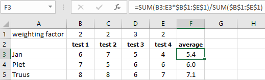
Figure 8.11: Weighted averages of test scores.

Calculate Jan’s weighted average by multiplying each test grade by its weighting factor and dividing the sum of these products by the sum of the weighting factors.
To make the formula copiable, determine which cell addresses should remain constant and make them absolute.

Formula F3: =SUM(B3:E3*$B$1:$E$1)/SOM($B$1:$E$1)

Then copy the formula to F4 and F5.

Task 8.6 File: Array5.xlsx

Figure 8.12 shows the gender and height (in cm) of several students. The average height for male and female students is calculated in cells C11 and C12.

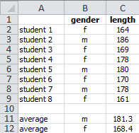
The array formula here is more complex because it needs to select heights based on gender. The IF function can achieve this.

Open the file.
Select cell C11 and enter the formula =AVERAGE(IF(B2:B9="m",C2:C9)).
Create a formula for cell C12 by adjusting the formula for female students.

Formula C12: =AVERAGE(IF(B2:B9="f",C2:C9))

8.4 Frequency Distribution

Use the FREQUENCY function to create a frequency distribution.

Syntax: FREQUENCY(data_array,bins_array).

The first argument is the array of values. The second argument is the array of bin boundaries for grouping the values. The result is an array of frequencies.

Task 8.7 File: Array6.xlsx

Open the file.
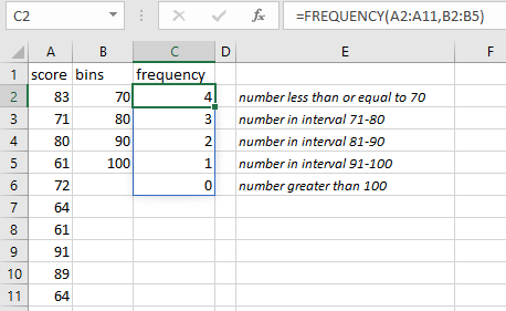
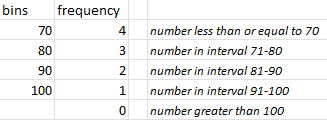
Enter the formula =FREQUENCY(A2:A11,B2:B5) in cell C2.

The result is a frequency table. Figure 8.14 explains how the interval boundaries are handled.

Figure 8.14: Explanation of frequency distribution intervals.

8.5 Dynamic Array Formulas

An array formula entered in one worksheet cell can output results into multiple cells. This is called spilling, and the output occupies a spill range. The number of cells in the spill range depends on the formula’s result. When the source data changes, the results update dynamically, and the spill range adjusts accordingly. A #SPILL! error occurs if other data obstructs the spill range.

To refer to a spill range, append a hash symbol # to the address of the first cell in the range. For example, if the spill range is J2:N4, refer to it as =J2#. This ensures that the reference adapts if the spill range’s size changes.

Naming arrays used in formulas can be very helpful. You can name them the same way you name individual cells.

Several new functions support dynamic array behavior: RANDARRAY, FILTER, SEQUENCE, SORT, SORTBY, UNIQUE, XMATCH and XLOOKUP.

8.5.1 RANDARRAY

Returns an array of random numbers. All arguments are optional.

Syntax

RANDARRAY([rows],[columns],[min],[max],[integer])

rows: The number of rows in the returned array (default is 1).
columns: The number of columns in the returned array (default is 1).
min: The smallest number to return (default is 0).
max: The largest number to return (default is 1).
integer: TRUE for integers, FALSE for decimals (default is FALSE).

Example 8.4 =RANDARRAY(3,4,10,50,TRUE)

Figure 8.15: Generates a 3x4 array with random integers between 10 and 50.

8.5.2 FILTER

Returns filtered values from an array or range.

Syntax

FILTER(array,include,[if_empty])

array: The range or array to filter.
include: An array of Boolean values (TRUE to keep a row/column, FALSE to exclude it).
if_empty: The value to return if no items are retained.

Example 8.5 File: Dynarray.xlsx

Extract rows where the gender is female.

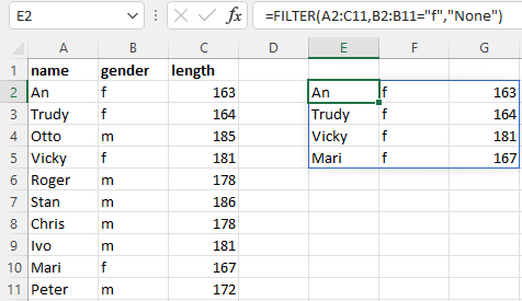
Figure 8.16: Filters a list of names to show only female entries.

To filter for males or unspecified genders, replace “f” with “m” or “z” in the formula.

You can also use multiple criteria. To filter for women shorter than 170 cm, use: =FILTER(A32:C41,(B32:B41="f")*(C32:C41<170),"None")

8.5.3 SEQUENCE

Returns a sequence of numbers based on a pattern.

Syntax

SEQUENCE(rows,[columns],[start],[step])

rows: The number of rows to return.
columns: The number of columns to return (default is 1).
start: The first number in the sequence (default is 1).
step: The increment between numbers (default is 1).

Example 8.6 =SEQUENCE(4,3,5,10)

Figure 8.17: Generates a 4x3 matrix of integers, starting with 5 and incrementing by 10.

8.5.4 SORT

Sorts the values in a range or array.

Syntax

SORT(array,[sort_index],[sort_order],[by_col])

array: The array to sort.
sort_index: The row or column number to sort by (default is 1).
sort_order: 1 for ascending, -1 for descending (default is 1).
by_col: TRUE to sort columns, FALSE to sort rows (default is FALSE).

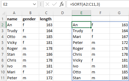
Example 8.7 File: Dynarray.xlsx

Sort an array by the values in column 3 (length).

Figure 8.18: Sorts an array by length (column 3).

8.5.5 SORTBY

Sorts a range or array based on the values in another range or array.

Syntax

SORTBY(array,by_array1,[sort_order], ...)

array: The array to sort.
by_array1: The array to sort by.
sort_order: 1 for ascending, -1 for descending (default is 1).

Example 8.8 File: Dynarray.xlsx

Sort names by length.

=SORTBY(A2:A11,C2:C11)

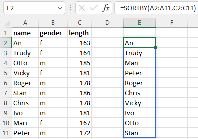
Figure 8.19: Sorts a list of names by length.

The array used for sorting doesn’t need to be included in the output.

You can also sort by multiple columns:

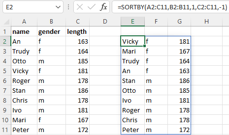
Example 8.9 File: Dynarray.xlsx

Sort the array by gender (ascending) and then by length (descending).

=SORTBY(A2:C11,B2:B11,1;C2:C11,-1)

Figure 8.20: An array is sorted ascending by gender, then descending by length.

8.5.6 UNIQUE

Returns an array with unique values from an array.

Syntax

UNIQUE(array,[by_col],[exactly_once])

array: The array to extract unique rows or columns from.
by_col: TRUE to return unique columns, FALSE to return unique rows (default is FALSE).
exactly_once: TRUE to return values that appear only once, FALSE to return all distinct rows or columns (default is FALSE).

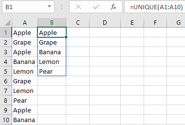
Example 8.10 UNIQUE(A1:A10)

Extracts the unique values from a list of names.

Figure 8.21: Extracts unique names from a list.

8.5.7 XMATCH

Searches for a value and returns its position within a row or column. This is a more advanced replacement for the MATCH function.

XMATCH supports approximate and exact matches, reverse searches, and wildcard characters (*?) for partial matches. Searches can start from the first or last value, and it also supports binary searches.

This function is often used with other functions. The XLOOKUP function is generally more useful.

Syntax

XMATCH(lookup_value,lookup_array,[match_mode],[search_mode])

lookup_value: The value to search for.
lookup_array: The array to search within.
match_mode: Specifies the type of match: 0 for exact match, -1 for exact match or next smaller item, 1 for exact match or next larger item, 2 for wildcard match (default is 0).
search_mode: Specifies the search direction: 1 to search from the first item, -1 from the last item, 2 for binary search (ascending), -2 for binary search (descending).

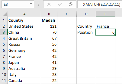
Example 8.11 =XMATCH(E1,A2:A11)

Finds the position of a country in the top 10 medal table from the 2016 Summer Olympics.

Figure 8.22: Finds the position of a country.

8.5.8 XLOOKUP

A modern and versatile replacement for VLOOKUP, HLOOKUP, and LOOKUP. It supports approximate and exact matches, wildcard characters (*?), and vertical or horizontal searches.

Syntax

XLOOKUP(lookup_value, lookup_array, return_array, [if_not_found], [match_mode], [search_mode])

lookup_value: The value to search for.
lookup_array: The array to search within.
return_array: The array to return values from.
if_not_found: The value to return if no match is found.
match_mode: Specifies the type of match: 0 for exact match, -1 for exact match or next smaller item, 1 for exact match or next larger item, 2 for wildcard match (default is 0).
search_mode: Specifies the search direction: 1 to search from the first item (default), -1 from the last item, 2 for binary search (ascending), -2 for binary search (descending).

Example 8.12 =XLOOKUP(D2,A2:A7,B2:B7,,-1)

Looks up the discount percentage based on the quantity in a discount table.

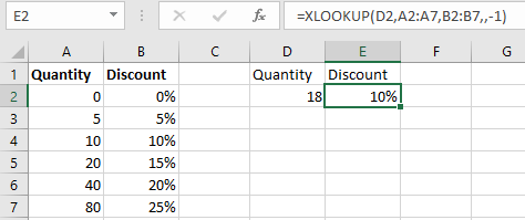
Figure 8.23: Determines the discount percentage.

ote the arguments in this formula:

lookup_value: D2
lookup_array: A2:A7
return_array: B2:B7
if_not_found: Not specified (hence the comma).
match_mode: -1
search_mode: Not specified (uses the default).

8.6 Tables and Array Formulas

Array formulas are often used with data lists, especially those with multiple columns. Using Excel tables with these formulas offers advantages: you can use table and column names in formulas, and references update automatically when rows are added or removed.

To refer to a column in an Excel table, use square brackets immediately after the table name: table_name[column_name].

Task 8.8 File: Personnel.xlsx

Open the file.
Convert the data range to a table using the Insert tab > Table, and name the table tblPersonnel.
Save the file as Personneltable.xlsx to preserve the original.
In a cell outside the data area (e.g., K4), enter the formula =UNIQUE(tblPersonnel[Department]).

This will create a list of department names. To sort this list alphabetically, nest it within the SORT function.

Change the formula to =SORT(UNIQUE(tblPersonnel[Department])).

This will give you a sorted list of department names.

Create a similar sorted list of division names.

8.7 Returning Multiple Values

XLOOKUP can return multiple values for a single match. This task demonstrates how to return four values with one formula.

Task 8.9 File: olympic2016.xlsx

Open the file.
Convert the data range to a table using the Insert tab> Table, and name the table Medals.
Add a Total column to the table with a formula to calculate the total number of medals:
- Enter the text Total in cell E1 and press ENTER to create a new column.
- In cell E2, type =SUM(, select cells B2:D2, type ), and press ENTER.

The total medal counts will appear in the Total column. Excel changes the formula in E2 to =SUM(Medals[@[Gold]:[Bronze]]).

Copy the texts in A1:E1 to G1:K1.
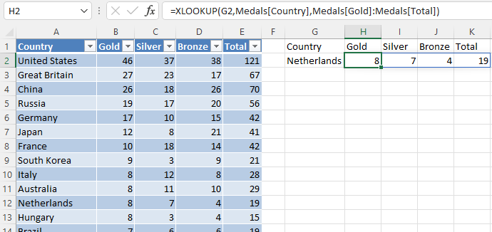
Enter the text Netherlands in cell G2.
SIn cell H2, enter the formula:
=XLOOKUP(G2,Medals[Country],Medals[Gold]:Medals[Total])

The result will look like this:

Figure 8.24: XLOOKUP returning multiple values.

8.8 Two-Way Lookup

XLOOKUP can also perform two-way lookups by nesting one XLOOKUP function within another.

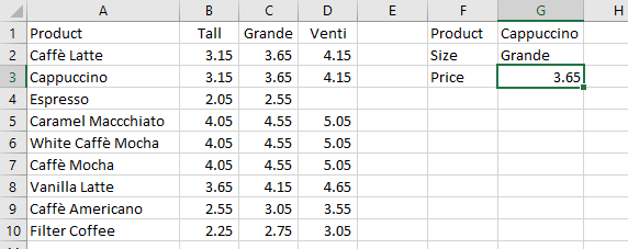
Figure 8.25 shows Starbucks coffee prices. Cell G3 should display the price based on the coffee type in G1 and the size in G2.

Figure 8.25: Nested XLOOKUP functions for a two-way lookup.

Task 8.10 File: Tidy001.xlsx

Open the file.
Enter the data in F1:F3 and G1:G2.
In cell G3, enter the formula:
=XLOOKUP(G2,B1:D1,XLOOKUP(G1,A2:A10,B2:D10)).

The inner XLOOKUP looks up the coffee type in the product column and returns a row of prices.
The outer XLOOKUP finds the correct size and returns the corresponding price.

8.9 Mathematical array functions

Linear algebra involves many arithmetic operations with arrays, and Excel provides specific functions for this. Their use is beyond the scope of this textbook.

MUNIT: Identity Matrix.; Returns the identity matrix for a given dimension. Primarily used with other matrix functions like MMULT.
MMULT: Matrix Multiplication.; Returns the matrix product of two arrays.
MINVERSE: Matrix Inverse.; Returns the inverse of a matrix, used for solving systems of equations. The product of a matrix and its inverse is the identity matrix.
MDETERM: Matrix Determinant.; Returns the determinant of a matrix, also used in solving systems of equations.

8.10 Exercises

Exercise 8.1 Array Addition (matr001)

Perform the following addition using array formulas.

Exercise 8.2 Failures per District (matr002)

File: Matr002.xlsx

A public utility company records gas, water, and electricity failures by district, as shown below. Calculate the total failures per district using array formulas.

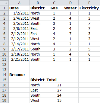
Enter array formulas in cells C16:C19 to calculate the total failures per district.

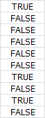
The formula (B2:B11)=B16 creates a 10-row column array. If a cell in B2:B11 equals B16 (“North”), the array value is TRUE (1); otherwise, it’s FALSE (0).

Multiplying this column array by {C2:E11} creates a 10-row, 3-column array. Rows multiplied by FALSE become zeroed; those multiplied by TRUE retain their original values.

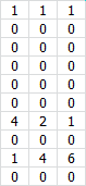
Summing all values in this array gives the total failures for the “North” district.

Exercise 8.3 Random Integers (matr003)

Use the RANDARRAY function to generate random numbers. Create a new file with the following data to experiment with dynamic array formulas:

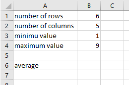
In cell B7, enter a formula to generate random integers, referencing cells B1:B4 for the arguments.
In cell B6, calculate the average of the generated numbers, referencing the spill range.
Experiment with different values in B1:B4. The maximum value must be greater than or equal to the minimum value.

Exercise 8.4 Random Dates and Times (matr004)

Excel stores dates and times as numbers. For example, 2020-06-30 18:00:00 is stored as 44012.75. The part before the decimal is the date, and the part after is the time. You can generate random dates and times using the RANDARRAY function.

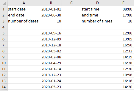
In a new worksheet, enter the data for the first three rows and apply the correct formatting.
In cell B5, enter a formula to generate dates, and in cell E5, a formula to generate times. Use the data in the first three rows as arguments. Apply date/time formatting to the spill ranges.
Experiment with different values in the first three rows. The maximum value must be greater than or equal to the minimum value.

Exercise 8.5 Sorting Columns (matr005)

File: Benelux-Population.xlsx

The figure shows the population of the Benelux countries for 2000, 2005, 2010, and 2015. Use the SORT function to display this data with the years in reverse order.

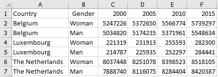
Open the file and copy the data in columns A and B to H and I, respectively. Enter the SORT formula in cell J1 to sort the data by year in descending order. The result should look like this:

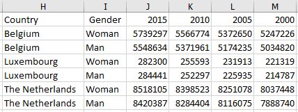
Save the file as matr005.xlsx to preserve the original.

Exercise 8.6 Sequence of Roman Numbers (matr006)

Create an array with the numbers 1 to 100 in a new worksheet, as shown below.

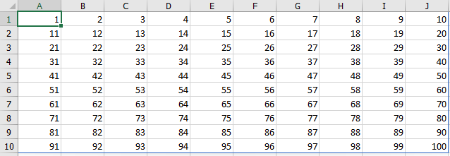
Then, modify the formula to display Roman numerals.

The ROMAN function converts Arabic numbers to Roman numerals (text).

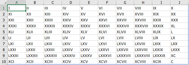
Save the file as matr006.xlsx.