4 Formatting Worksheet and Data
- The importance of selecting fbefore formatting.
- Adjusting column width and row height.
- Formatting numbers and text.
- Predefined formatting styles.
- Copying cell formatting.
- Conditional formatting.
Excel provides many options to change the appearance of a worksheet and the data in its cells, enhancing readability and presentation.
You can apply formatting (e.g. font type) to the entire worksheet, individual cells, or cell ranges. The process is generally the same but depends on the selection.
Always select first, then apply the format.
To select the entire worksheet, click the button to the left of the first column and above the first row: 
4.1 Column Width
A column might be too narrow to display the entire cell content. If the content is text, you’ll only see the portion that fits. If it’s a number, you’ll see hash marks: ####.
Column width can be set from 0 to 255, representing the number of characters that fit in a cell with the default font. The default column width is 8.43, or about eight characters in the default font. A width of 0 hides the column.
You can adjust column width in several ways:
Double-click the right edge of the column header. The column width automatically adjusts to the longest text in the column.
Drag the column edge: Position the mouse pointer over the right edge of the column header, press and hold the left mouse button, and drag the edge to the desired width. Excel displays the current width in a small tooltip while dragging.
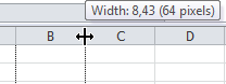
Figure 4.1: Adjusting column width through dragging Use the Column Width dialog box: Right-click the column header and select Column Width from the context menu. Enter the desired width and click OK.
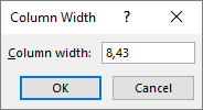
Figure 4.2: Specifying column width Use the Home tab: Select a cell in the column you want to adjust Then, choose Home > Format (group Cells) > Column Width…. This opens the same dialog box.
To adjust multiple columns simultaneously, select them using the SHIFT-key or CTRL-key.
To change the width of all columns in the worksheet, use Home > Format (Cells group) > Default Width...
4.2 Row Height
Row height usually adjusts automatically to fit the data. However, you might need to adjust it for formatting purposes. Row height can range from 0 to 409, measured in points (1 point is about 0.035 cm). The default row height is 12.75 points (about 0.4 cm). A row height of 0 hides the row.
You can adjust row height in several ways:
Double-click the bottom edge of the row header. The row height automatically adjusts to fit the content.
Drag the row edge: Position the mouse pointer over the bottom edge of the row header, press and hold the left mouse button, and drag the edge to the desired height. Excel displays the current height in a tooltip while dragging.
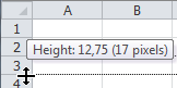
Figure 4.3: Adjusting row height through dragging Use the Row Height dialog box: Right-click the row header and select Row Height… from the context menu. Enter the desired height and click OK.
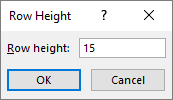
Figure 4.4: Specifying row height Use the Home tab: Select a cell in the row you want to adjust. Then, choose Home > Format (Cells group) > Row Height…. This opens the same dialog box.
To adjust the height of multiple rows at once, select them using the SHIFT-key or CTRL-key .
4.3 Font
The Font group (Home tab) provides commands to change the appearance of text in cells. To apply these changes, first select the cell(s) and then use the command button. The options in this group are:
 : A dropdown list to choose the font.
 : A dropdown list to choose the font size.
 : Increases or decreases the font size in 2-point increments.
 : Toggles Bold, Italic, or Underline. The underline style can be specified using the dropdown arrow.
 : A dropdown palette to choose the font color.
 : A dropdown palette to choose the cell background color.
4.4 Cell Borders
Borders are often used to visually group cells, such as placing a line above a total. Borders enhance the layout of a worksheet.
To add borders to cells:
Select the cell(s).
Choose Home > Borders dropdown arrow (Font group).

Choose the desired border style from the list.
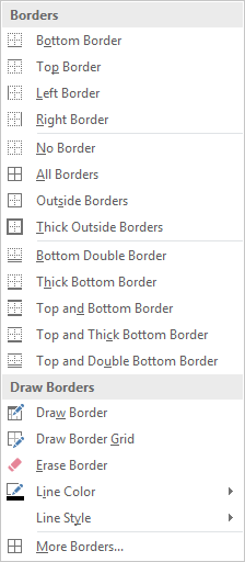
If the desired border style isn’t in the list, click More Borders…. This opens the Format Cells dialog box with the Border tab selected.
4.5 Cell Alignment
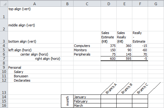
Cell alignment controls how content is positioned within a cell, both horizontally and vertically. By default, content is bottom-aligned vertically. Text is left-aligned, numbers are right-aligned, and logical values (TRUE or FALSE) are center-aligned horizontally. You can change these defaults, as shown in Figure 4.6.
To apply specific alignment, first select the cell(s) and then click an alignment button in the Home > Alignment group.
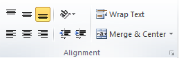
The buttons are self-explanatory; tooltips appear when you hover over them.
The example uses these options:
- Vertical alignment
-
Options are top, middle, and bottom (cells A1:A3).
- Horizontal alignment
-
Options are left, center, and right (cells A5:A7).
- Indentation
-
Options are increase indent and decrease indent (cells A10:A12).
- Orientation
-
Predefined rotation options (cells D13:F13 and B14).
- Wrap Text
-
Displays text on multiple lines within a cell, increasing row height and reducing horizontal space (cells D3:F3).
If all wrapped text isn’t visible, the row might be set to a specific height. To allow the row to adjust automatically, choose Home > Format (group Cells) > AutoFit Row Height.
- Merge & Center
-
Combines selected cells into a single larger cell and centers the content. Often used for titles that span multiple rows or columns. Cells can be merged horizontally and vertically (cells B14:B16).
4.6 Formatting Numbers
Numbers can be displayed in various formats, including with or without decimal places, currency symbols, and date or time separators. You can also create custom formats.
Excel automatically formats some numbers as you enter them:
Typing 19% displays the number as 19% (right-aligned), but the cell content is 0.19.
Typing €123,45 displays it as € 123,45 (right-aligned), and the cell content is 123,45.
Typing 1/2 displays it as a date (e.g., 2-Jan).
Excel stores dates and times as serial numbers, starting with January 1, 1900, as 1. So, 1/2 becomes a date, and the cell content is a serial number representing that date (e.g., 41276).
To quickly format numbers, use the commands in the Number group (Home tab).
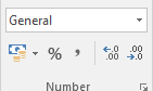
Common formatting buttons include:
 : Accounting Number Format, adds a currency symbol (dropdown arrow for options).
 : Percent style, formats as a percentage
 : Comma style, adds a thousands separator.
 : Increase Decimal, adds decimal places.
 : Decrease Decimal, removes decimal places.
The current cell format is displayed at the top (e.g., “General”), with a dropdown arrow for predefined styles.
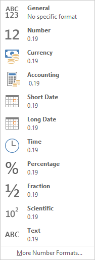
For more control, click More Number Formats… to open the Format Cells dialog box with the Number tab selected, where you can define custom formats.
This example shows various number formatting options:
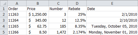
Task 4.1 File: Numberformat.xlsx
Open the file.
Format the worksheet as shown, using the Number group (Home tab) options.
- Column A: Numbers formatted as text.
- Column B: Accounting number format.
- Column C: Numbers with thousands separator and 0 decimal places.
- Column D: Numbers entered with percent sign, adjusted decimal places.
- Column E: Dates, short date format for the first two, long date format for the last two.
4.7 Copying and clearing Formats
Cell format and content are stored separately, allowing you to copy or delete them independently.
Copying format
The fastest way to copy a cell’s format is using the Format Painter button.
To use it:
- Select the cell with the desired format.
- Choose Home >
 (Clipboard group). The mouse pointer changes to a brush (
 ).
). - Select the destination cell(s).
- Release the mouse button.
Double-clicking the Format painter button allows you to apply the format to multiple cells. Press Esc or click the Format painter button again to cancel.
Clearing Formats
To remove cell formatting:
Select the cell(s).
Choose Home > Clear (group Editing) > Clear Formats.
You can clear the format, content, or both.
The DELETE key only clears the cell’s content, not its formatting.
4.8 Table Styles
To practice formatting a list using predefined styles:
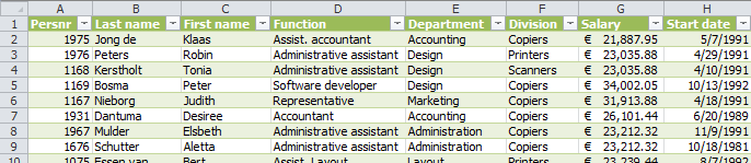
Task 4.2 File: Personnel.xlsx
Open the file.
Select any cell within the data area.
Choose Home > Format as Table (Styles group).
Select a style, e.g. Table Style Medium 4.
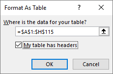
- Click OK.
4.9 Conditional Format
Conditional formatting applies formatting to cells based on specific conditions. For example, you can highlight cells with values less than 6 in red. The formatting is applied when the condition(s) are met; otherwise, the “regular” format is used.
Conditional formatting can use number formats, fonts, borders, and background colors.
Conditions can compare cell values to a fixed value, a range of values, or other criteria like deviation from the average or the top/bottom values. You can apply multiple conditions.
4.9.1 Formatting with One Condition
A teacher wants to highlight failing grades (less than 6) in light red.
Task 4.3 File: Marks.xlsx
Open the file.
Select all the grades.
Choose Home > Conditional Formatting (group Styles) > Highlight Cells Rules > Less Than… and enter the condition and format.
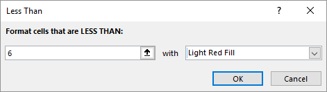
- Click OK.
Failing grades are now highlighted in light red.
Test the formatting by changing some grades; the background color should update accordingly.
4.9.2 Formatting with Two Conditions
A sales report tracks achieved and target turnover. The task is to color-code the turnover: green if the target is met, red if not.
Task 4.4 File: Turnover-Q1.xlsx
Open the file.
Select all the turnover data, cell C2 through cell C15.
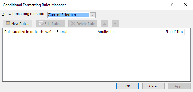
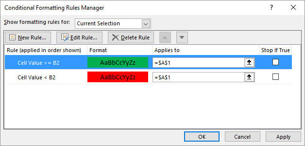
Choose Home > Conditional Formatting (Styles group) > Manage Rules….
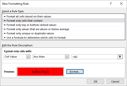
Click New Rule…. The New Formatting Rule dialog box appears.
Select Format only cells that contain, set Cell Value to less than
=B2and choose a red fill color as the format.
Click OK. The Conditional Formatting Rules Manager reappears.
Click New Rule and create another rule:
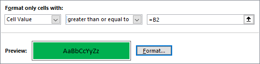
- Click OK. The manager now shows both rules:
- Click OK.
The formatting is applied.
Test the formatting by changing values to ensure the colors update.
4.9.3 Formatting Top/Bottom 10%
You can create conditions based on a range of values, such as the top/bottom 10% or top/bottom 3 values.
For a car dataset, the task is to highlight the 10% of cars with the lowest fuel consumption in green.
Task 4.5 File: Car.xlsx
Open the file.
Select the fuel consumption values (column F).
Choose tab Home > Conditional Formatting (Styles group) > Top/Bottom Rules > Bottom 10%… and set the values in the dialog box.
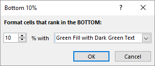
- Click OK.
4.9.4 Removing Conditional Formatting
To remove conditional formatting:
Select the cell(s).
Choose tab Home > Conditional Formatting (Styles group) > Clear Rules > Clear Rules from Selected Cells.
4.9.5 Finding Conditional Formatting
To find cells with conditional formatting:
Choose tab Home > Find & Select (Editing group) > Conditional Formatting.
Excel selects all cells with conditional formatting or displays “No cells were found.”