5  Modeling Calculations

OBJECTIVES

• Create formulas.
• Set up a calculation model.
• Copy formulas and understand absolute and relative cell addresses.
• Create formulas that evaluate to TRUE or FALSE.
• Naming cells and use the names.

One of the most important aspects of working with Excel is performing calculations, which requires using formulas. To work effectively and efficiently with formulas, it’s crucial to plan the worksheet layout carefully. This can save significant time and effort.

Calculations are performed using formulas. Formulas contain numbers or references to cells containing numbers. Operators, such as +, -, *, /, and ^, indicate the type of calculation.

A formula must always begin with the = character. While you can start a formula with a +, Excel will automatically convert it to = after you enter the data.

To enter a formula, start by typing =, then enter the calculation as you would on a calculator. Instead of numbers, you can use cell addresses or cell names that refer to cells containing numbers. You can also select cell addresses with the mouse instead of typing them.

Table 5.1 shows the symbols (operators) used in calculations.

Table 5.1: Operators.

Symbol	Meaning	Example	Result
+	Addition	=4+5	9
-	Subtraction	=29-6	23
*	Multiplication	=7*8	56
/	Division	=6/2	3
^	Exponentiation	=2^3	8
()	Parentheses for operator precedence	=30-(4+6)	20

Task 5.1 Practice with these examples in a worksheet.

5.1 Your First Formulas

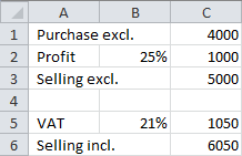
This exercise demonstrates a simple calculation, as shown in Figure 5.1. The worksheet contains three input values:

• C1: Purchase amount
• B2: Profit margin
• B5: VAT rate

Cells C2, C3, C5, and C6 contain formulas that automatically update when you change the values in C1, B2, or B5.

Figure 5.1: Example calculation purchase, profit and selling.

Task 5.2 Calculate Sellings

1. Create a new worksheet in a new workbook.

2. Enter the text labels shown in column A. Don’t worry if some text extends beyond the column width for now. You can adjust the column width later if desired.

3. Enter the following values:

   • B2: 25%
   • B5: 21%
   • C1: 4000

4. In cell C2, enter the formula =B2*C1. After pressing Enter, the result (1000) appears in C2 (the calculated profit).

5. In cell C3, enter the formula =C1+C2. The result (5000) appears in C3.

6. In cell C5, enter the formula =B5*C3. The result (1050) appears in C5.

7. In cell C6, enter the formula =C3+C5. The result (6050) appears in C6.

8. Experiment by entering different values for the purchase amount, profit margin, and VAT rate.

Observe how all the calculated values update automatically.

5.2 More with Formulas

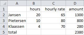
The worksheet in Figure 5.2 calculates wages by multiplying hours worked by an hourly rate. The total wages are calculated by adding individual wages.

Figure 5.2: Example calculation hours, hour rate and totals.

Task 5.3 File: Wages.xlsx Calculate Working Hours

1. Open the file.

2. Enter the correct formulas in the “Amount” column:

   • D2: =B2*C2
   • D3: =B3*C3
   • D4: =B4*C4
   • D5: =D2+D3+D4

5.3 Calculation Models

Excel can perform a wide variety of calculations. Designing effective calculation models, especially for larger and more complex tasks, requires careful planning.

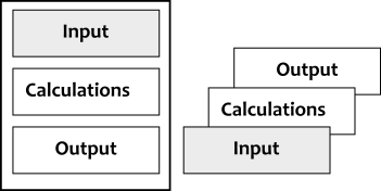
A calculation model typically involves three types of cells:

Input

Cells where users enter variable values.

Calculations

Cells containing formulas that perform calculations using the input values.

Output

Cells that display the formatted results of the calculations.

The data flow in a model progresses from input to calculations and then to output. However, it’s often best to plan the model in reverse: start with the desired output, then determine the necessary calculations, and finally identify the required input.

Here are some guidelines for designing calculation models in Excel:

1. Separate Input, Calculations, and Output:

   • For smaller models, you can use different sections within a single worksheet (e.g., input at the top).

   • For larger models, use separate worksheets for each type of cell.

Figure 5.3: Design of a calculation model.At the left 1 worksheet, at the right 3 worksheets.

2. Organize Worksheets Logically:

   • Design worksheets to be read from top to bottom and left to right, like a book.

3. Identify Variables:

   • Place changeable values (e.g., item prices) in individual cells. These values are the model’s variables.

4. Use Cell References in Formulas:

   • Minimize the use of direct numbers in formulas. Instead, refer to cells containing those numbers. This also applies to values that change infrequently, such as a VAT rate.

5. Label Cells Clearly:

   • Provide explanatory text in adjacent cells (to the left or above) to describe the purpose of cell content.

6. Use Headers:

   • Include headers above columns and to the left of rows containing numbers.

7. Standardize Formulas:

   • If possible, use similar formulas within a row or column to facilitate copying.

8. Break Down Complex Formulas:

   • Divide complicated formulas into smaller parts to calculate and check intermediate results (e.g., subtotals). This helps prevent errors.

9. Name Worksheets Appropriately:

   • Use descriptive names for worksheets in models with multiple sheets.

10. Document Your Model:

    • Include documentation, especially for larger models, in separate worksheets.

5.4 Copying Formulas

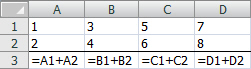
Copying formulas to other cells is very useful, especially when the formulas are similar. In @fig-formula-copy, the formulas in A3, B3, C3, and D3 are nearly identical. You can enter the formula once in A3 and then copy it to B3:D3.

A (cell)range is a group of cells that you can refer to in a formula. Ranges are typically rectangular and defined by the cell in the upper-left corner, a colon, and the cell in the lower-right corner (e.g., B2:E7, B3:E3, D2:D6).

Figure 5.4: Example with copyable formulas.

Since formulas often contain cell references, it’s important to understand how these references behave when you copy a formula. There are two types of cell references:

• Relative: Cell references adjust to their new location.

• Absolute: Cell references remain fixed.

Use dollar signs ($) to make a cell reference absolute. You can make the column letter, the row number, or both absolute. Table 5.2 shows the different possibilities.

Table 5.2: Examples of cell addresses.

Type	Example
Relative address	B1
Absolute column and absolute row address	$B$1
Absolute column and relative row address	$B1
Relative column and absolute row address	B$1

When you copy a formula, the absolute parts of cell references remain unchanged, while the relative parts are adjusted.

You can change the type of cell reference in these ways:

• Type the dollar signs directly in the cell address.

• Place the cursor within the cell address and press the F4 key repeatedly to cycle through the four reference types.

5.4.1 Copy Rules

When you copy formulas with cell references, Excel applies these rules:

• When copying to the left or right, the column letter changes.

• When copying up or down, the row number changes.

• Parts of the address with a dollar sign ($) remain unchanged.

Table 5.3: Examples of copy actions.

Formula	Copy action	Result
=A1+B2	1 cell to the right	=B1+C2
	1 cell down	=A2+B3
	1 cell to the right and 1 cell down	=B2+C3
=A$1+B$2	1 cell to the right	=B$1+C$2
	1 cell down	=A$1+B$2
	1 cell to the right and 1 cell down	=B$1+C$2
=$A1+$B2	1 cell to the right	=$A1+$B2
	1 cell down	=$A2+$B3
	1 cell to the right and 1 cell down	=$A2+$B3
=$A$1+$B$2	Any copy action	=$A$1+$B$2

5.4.2 Premium Table

The worksheet in Figure 5.5 shows a list of car insurance premiums. The list starts with a value of $10,000 and a premium of $675. Subsequent values increase in increments of $1,000, and the premium increases by $45. Use formulas to create this list for rows 6 through 20.

Figure 5.5: Premium table.

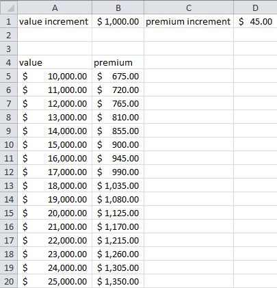
Task 5.4 File: Premium-Table.xlsx

1. Open the file.

2. Format the values as currency using Home > button Accounting Number Format (group Number). Adjust the column widths to display all content.

3. In cell A6, enter the formula =A5+$B$1.

4. In cell B6, enter the formula =B5+$D$1.

5. Select the range A6:B6 and drag the fill handle to row 20.

5.5 True/False Formulas

Some formulas don’t perform calculations but instead compare values or test conditions. These formulas, also called Boolean expressions, return either TRUE or FALSE.

Table 5.4 lists the operators used in Boolean expressions.

Table 5.4: Operators for comparing two items.

Operator	Meaning
=	Equal to
<>	Not equal to
<	Less than
<=	Less than or equal to
>	Greater than
>=	Greater than or equal to

Table 5.5 provides examples of Boolean formulas. To understand how they work, you can enter them into cells in a worksheet. The parentheses in the formulas are not strictly required but improve readability, so it’s recommended to use them.

Table 5.5: Examples of TRUE/FALSE formulas.

Formula	Result
=(1=1)	TRUE
=(1=2)	FALSE
=(1<>1)	FALSE
=(1<>2)	TRUE
=(1<1)	FALSE
=(1<2)	TRUE
=(1<=1)	TRUE
=(1<=2)	TRUE
=(1>2)	FALSE
=("a"="b")	FALSE
=("a"<>"b")	TRUE

Always enclose text in double quotes in Boolean operations.

Using Boolean formulas directly in cells isn’t very practical. However, they are powerful within calculations. Excel treats TRUE as 1 and FALSE as 0, allowing you to perform calculations based on conditions.

In the following example, the shipping cost for an order depends on the order amount.

Example 5.1 Calculate Shipping Costs

An online shop offers free shipping for orders of $25 or more. The following figure shows how a Boolean formula calculates the shipping cost. The formula (B5<$B$2) returns TRUE (1) if the order total (B5) is less than $25 (B2) and FALSE (0) otherwise. This result is then multiplied by $3.50, resulting in either $3.50 or $0.

Figure 5.6: Example with a true/false formula.

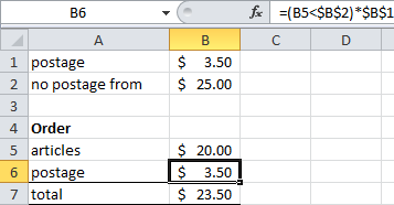
Create this example and verify its functionality by entering different values in cells B1, B2, and B5.

5.6 Cell Names

This section describes how to use meaningful names for cells and the rules for naming them.

Using cell addresses in formulas can make them confusing and difficult to read, obscuring the formula’s purpose. Fortunately, you can assign descriptive names to cells and ranges, allowing for more intuitive formulas like =Sales-Purchases.

Naming Rules:

• Names must begin with a letter or an underscore (_). Subsequent characters can be letters, numbers, or underscores. Names cannot start with a number.

• Names cannot contain spaces. Use underscores to simulate spaces (e.g., Sales_2010).

• Most symbols (commas, colons, exclamation points, etc.) are not allowed.

5.6.1 Creating Names

You can assign names to cells in several ways. The preferred method often depends on user preference and typing speed. This task presents two methods for assigning names and three methods for using names in formulas. You can use the same methods to name cell ranges.

Task 5.5  

1. Create a new worksheet.

2. Enter 100 in cell A1 and 275 in cell A2.

3. Select A1 and choose Formulas > Define Name (Defined Names group).

Figure 5.7: Dialog box New Name.

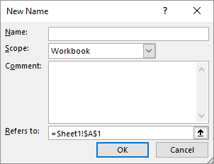
In the Name text box, you can enter the desired name. Excel may suggest a name. The optional Comment box allows you to provide a description for future reference (e.g., for audits or documentation).

4. Enter Purchases as the name and click OK. The name box now displays “Purchases” instead of the cell address.

Figure 5.8: Cell A1, now with the name Purchases in the name box instead of the address.

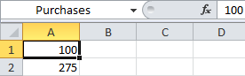
An alternative and faster way to name a cell is to enter the name directly in the name box. The next step demonstrates this for cell A2.

5. Select cell A2. Click in the Name box, replace A2 with Sales, and press Enter.

6. Select cell A3 and enter the formula to calculate profit using one of these methods:

   • Type = Sales-Purchases and press Enter.

   • Type =, select A2, type -, select cell A1 and press Enter.

   • Type =, choose Formulas > Use in formula (group Defined Names) > Sales, type -, choose Formulas > Use in Formula (Defined Names group) > Purchases and press Enter.

Cell A3 will display 175. Selecting cell A3 will show =Sales-Purchases in the formula bar, demonstrating the improved readability of formulas with names.

5.6.2 Using Names in Existing Formulas

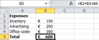
When you assign a name to a cell or cell range, Excel automatically uses those names in new formulas, but not in existing ones. For example, if cell B5 contains the formula =B2+B3+B4, and you then assign names to cells B2, B3, and B4, the formula in B5 remains unchanged.

Figure 5.9: Formula with addresses instead of names.

However, you can easily replace the cell addresses in existing formulas with the newly assigned names. In the example file, the cells used in the formula already have names. The following steps demonstrate how to replace the addresses in the formula with those names.

Task 5.6 File: Office-Expenses.xlsx

1. Open the file.

2. Select cell B5.

3. Choose Formulas, click the arrow on the Define Name (Defined Names group) button and select Apply Names.

Figure 5.10: Dialog box apply names.

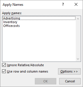
4. Select all names and click OK. The formula in cell B5 will change to =Inventory+Advertising+Officecosts.

To select multiple names, hold down the Ctrl key.

5.6.3 Managing Names

Excel provides tools for managing names, including viewing a list of all names in the workbook, and changing or deleting names. These tools are essential for managing names, especially in larger workbooks with many named cells and ranges.

Task 5.7 File: Expenses.xlsx

1. Open the file.

2. Choose Formulas > Name Manager (Defined Names group).

Figure 5.11: Name Manager.

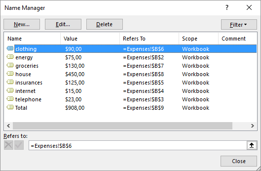
The Name Manager dialog box allows you to perform several operations:

• Deleting aname: Select the name and click Delete.

• Edit a name: Select the name and click Edit.

• Add or edit a comment: Select the name and click Edit.

• Create a new name: Click New.

5.6.4 Documenting Names

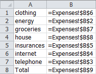
It’s helpful to create a list of all defined names and their corresponding cell addresses for documentation purposes. Excel can generate this list on a worksheet, although the procedure is not immediately obvious. It’s recommended to create the list on a new worksheet.

Task 5.8 File: Expenses.xlsx

1. Open the file.

2. Create a new sheet and select cell A1.

3. Choose Formulas > Use in formula (Defined Names group) > Paste Names > Paste List.

Figure 5.12: List of cell names and addresses.

5.7 Case Study: Price Calculation for Items

This case study demonstrates creating a calculation model using formulas and copying formulas.

An airport shop sells items both tax-free and with 21% VAT. Tax-free prices are in U.S. dollars, but customers can pay in euros. Prices with VAT are always in euros. Figure 5.13 shows a portion of the price table. The item numbers and dollar prices are simplified for practice purposes. The goal is to create this table efficiently. Only general guidance is provided, not detailed steps.

Figure 5.13: Price table

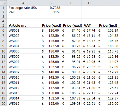
1. The dollar exchange rate and the VAT percentage are input variables and should be placed at the top of the worksheet, separate from the price table. Include explanatory labels in the adjacent cells.

2. The item numbers follow a pattern. Enter the first two numbers, select them, and drag down to generate the rest.

3. The dollar prices also follow a pattern (increments of 2.50). Enter the first two prices, select them, and drag down. Format the prices as currency with two decimal places and the dollar sign ($) symbol.

4. Calculate the price in euros by multiplying the dollar price by the dollar exchange rate. Enter the formula in the first cell (C6) and copy it down. Use an absolute reference for the dollar exchange rate so it doesn’t change when you copy the formula.

5. Calculate the VAT amount by multiplying the euro price by the VAT rate. Calculate the price including VAT by adding the VAT amount to the euro price. Enter the formulas in the first cells (D6 and E6) and copy them down. Use an absolute reference for the VAT rate.

6. Format all euro amounts as currency.