14 Goal Seek
- Understand the Goal Seek method.
- Identify applications for Goal Seek.
- Learn tips for using Goal Seek effectively.
A formula consists of one or more variables. Typically, you want to know the result of the formula for specific variable values. However, sometimes the reverse is true: you have a desired outcome and need to find the variable values that achieve it.
When a formula’s outcome depends on only one variable, you can use the Goal Seek method. This method iteratively changes the variable’s value until the formula produces the desired result.
If a formula’s outcome depends on multiple variables, you should use Excel’s Solver add-in.
Goal Seek Dialog Box
Goal Seek can be accessed via Data tab> What-If Analysis (Forecast group) > Goal Seek.
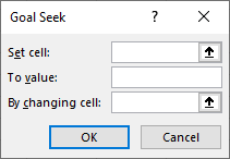
In the dialog box, you need to specify three values:
- Set cell
-
The cell address containing the formula for which you want a specific result.
- To value
-
The desired outcome of the formula; in other words, your goal.
- By changing cell
-
The cell address whose value Excel should change to achieve the target. This cell contains the variable.
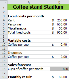
14.1 Break-Even Analysis for a Coffee Stand
Suppose you want to operate a coffee stand in a soccer stadium. You know the monthly costs for rent, staff, and miscellaneous expenses, as well as the cost and selling price of a cup of coffee. A calculation model has been created to determine the monthly profit or loss, as shown in Figure 14.2, based on the number of cups of coffee sold.
- Information needed
-
How many cups of coffee do you need to sell per month to break even?
In this simple example, you could easily calculate the answer manually. However, Goal Seek is well-suited for such problems.
Task 14.1 File: Stadium_Coffee.xlsx
Open the file.
Choose Data tab> What-If Analysis (Forecast group) > Goal Seek.
Specify the values for Goal Seek.
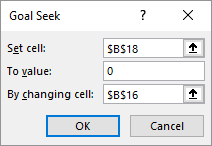
Set cell: The cell with the monthly result, B18.
To value: Zero, for break-even.
By changing cell: The cell with the number of cups of coffee to be sold, B16.
- Click OK.
Excel will start calculating and find the value 562.5. Since you cannot sell half cups of coffee, you will need to round the answer up to 563.
14.2 Tips for Using Goal Seek
It’s possible that the formula is structured such that the desired answer doesn’t exist. It’s also possible that an answer exists, but Excel cannot find it. In such cases, a dialog box will appear indicating this.
If a solution exists but Excel cannot find it, check the following:
Verify in your model that the result cell (Set cell) actually depends on the changing cell. The result cell must always contain a formula or function.
Ensure that the cell to be changed (By changing cell) contains only a value, not a formula or function.
Try different initial values in the cell to be changed.
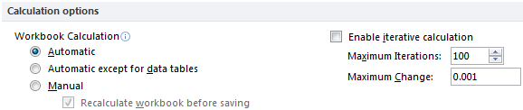
Increase the maximum number of iterations (default is 100) via File > Options > Formulas, as shown in Figure 14.4.
14.3 Exercises
Exercise 14.1 Freelancer Earnings (goal001)
Suppose you want to work as a freelancer but only if you can earn at least $5,000 per month. You receive a commission of 7.8% for each project.
Create a model in a worksheet where you can enter total sales and the commission percentage. Calculate the commission amount.
Use Goal Seek to determine the total sales required to achieve a commission of $5,000.
Total sales $ 64,102.56
Exercise 14.2 Loan Payment Calculation (goal002)
Using the PMT function, you can calculate the periodic payment for a loan based on constant payments and a constant interest rate. The following illustration is an example of such a calculation. Payments are made at the beginning of each period, and the loan is fully paid off after the last term.
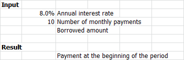
PMT function.- Recreate this model in a worksheet.
- Use Goal Seek to determine how much you can borrow if your maximum monthly payment is $750.
Since a payment is a cash outflow, the result of the PMT function is typically a negative number.
Loan amount $ 7280.
Exercise 14.3 Break-Even Point Analysis (goal003)
An entrepreneur faces costs and revenues that depend on the production quantity, Q. The relationships are as follows:
Total Costs (TC): \(Q^2 + 8Q + 15\)
Total Revenues(TR): \(-5Q^2 + 80Q\)
The following chart plots TC and TR as a function of Q.
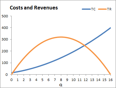
- Recreate this chart.
- Determine the break-even point(s). This is the quantity Q where costs equal revenues (TC = TR). The chart shows two such points. Use Goal Seek to find both solutions, providing answers to four decimal places.
Solution 1: Q=0.2120 and TC=TR=16.74
Solution 2: Q=11.7879 and TC=TR=248.26
Exercise 14.4 Savings Account Growth (goal004)
On January 1, 2010, an amount of $1,000 is deposited into a savings account. The account earns 2.7% annual interest, which is added to the principal. The following table shows the growth of the savings account balance over the first ten years.
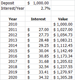
- Create this model in a worksheet.
- Use Goal Seek to determine the initial deposit required to have $2,500 in the savings account after 10 years.
Initialdeposit $ 1915.29.