3 Data Entry and Editing
- Entering data.
- Language dependent number separators.
- The difference between content and formatting of a cell.
- Inserting rows and columns.
- Copying data to other places
- Entering data conntaining a pattern.
Entering data (text, numbers, formulas) is one of the main activities in Excel. In short, it involves:
- Select a cell.
- Start typing.
- Press the Enter key.
Be aware that if the cell already contains content, this content will be overwritten.
After you press the Enter key, the cell cursor automatically moves down one cell.
3.1 Language-dependent number formats
Separators for decimals and thousands depend on the Windows language settings but can be changed in Excel. By default, Excel uses the number formats defined in Windows, with these characters:
- English
-
Decimal separator period (
12.34) -
Thousands separator comma (
12,345) - Dutch
-
Decimal separator comma (
12,34) -
Thousands separator period (
12.345)
To change these settings permanently, you must do so through the regional settings in the Windows Control Panel.
You can temporarily change these settings in Excel. To do this:
- Click File > Options > Advanced
- In the “Editing options” section , uncheck Use system separators.
- Enter the new separator in the Decimal separator and Thousands separator boxes.
To revert to the system separators, check the Use system separators box again.
3.2 Data entry examples
A simple exercise in data entry.
Task 3.1
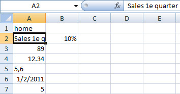
Select cell A1.
Type
homeand press Enter.
The word “home” is left-aligned in the cell and the active cell moves down to A2.
- Type
Sales 1e quarterand press Enter.
The text is left-aligned and appears to extend beyond the cell boundaries. However, the text is fully contained in cell A2; it only appears to overlap cell B2 because B2 is empty. The active cell is now A3.
- Type
89and press Enter.
The number is right-aligned in cell A3. The active cell is now A4.
- Type
12.34and press Enter.
The number is right-aligned in cell A4. The active cell is now A5.
- Type
5,6and press Enter.
The content of cell A5 is left-aligned. The comma causes Excel to interpret the entry as text, which is why it’s left-aligned. The active cell is A6.
- Type
1/2/2011and press Enter.
The date is right-aligned. Excel interprets dates as numbers and applies a special date format. The active cell is now A7.
- Type
=2+3and press Enter.
The cell displays the number 5. Excel interprets entries starting with = as formulas, calculates the result, and displays it. The cell’s content is the formula, not the result. The active cell is now A8.
- Select cell B2, type
10%and press Enter.
The content in cell B2 is right-aligned. The percent sign tells Excel to interpret the data as a number. The actual content of this cell is 0.1, which is formatted and displayed as a percentage. Because cell B2 is no longer empty, the full text in cell A2 is now truncated in the display.
- Select cell A2.
The formula bar shows the complete text entered in the cell.
You can adjust the column width to display all the text in cell A2.
Summary
- Text is left-aligned by default.
- Numbers are right-aligned by default.
- Commas and periods have different meanings in numbers.
- Formulas always begin with the
=character. - Dates are treated as numbers and formatted as dates.
- Numbers with a percent sign are treated as numbers and formatted as percentages. The cell content is the numerical equivalent (e.g., 10% is stored as 0.1).
- A cell has content and a format. What you see isn’t always the actual content.
3.3 Editing cell content
You can edit cell data in one of these ways:
- Double-click the cell. The cursor appears in the cell, allowing you to edit the content directly.
- Select the cell and press F2. The cursor moves to the end of the cell content for editing.
- Select the cell and click in the formula bar to position the cursor for editing.
When a cell is in edit mode, the status bar (bottom left) changes from “Ready” to “Edit.” Three icons also appear to the left of the formula bar:
![]()
These icons allow you to undo, confirm, or insert a function.
You must presse Enter to finalize changes and return to “Ready” mode.
3.4 Undoing changes
You can undo most actions in Excel using the Undo and Redo buttons on the Quick Access Toolbar.
 Undo
Undo-
Reverses the last action. Clicking it repeatedly undoes previous actions. The dropdown arrow next to the button displays a list of recent actions. Clicking an action in the list undoes all actions up to and including that one.
 Redo
Redo-
Reverses the effect of the Undo action. The dropdown arrow (if available) shows a list of undone actions that can be redone.
3.5 Inserting rows and columns
You’ll often need to insert rows or columns within existing data. The process is the same for both.
- Right-click the row or column header.
- Choose Insert.
To insert multiple rows or columns, select the desired number of rows/columns, right-click, and select Insert. The new rows or columns are inserted before the first row or column of your selection.
3.6 Copy and Paste
Copying cell content is a common task in Excel. You can copy a single cell or an entire range. By default, Excel copies both the content and formatting of the cells. However, you can choose to copy only the content or only the formatting. When you copy a formula with cell references, the references adjust to the new location.
Task 3.2 File: Cellformat.xlsx
- Open the file.
- Select the range A1:B13.
- Choose Home > Copy (Clipboard group).
- Select the upper-left cell of the destination, for example, D20.
- Choose Home > Past (Clipboard group.
3.7 Auto fill
How to quickly enter data that follows a pattern.
Excel provides several ways to quickly fill rows or columns with data that follows a pattern or is based on a list. Excel has built-in lists for days of the week and months of the year, and you can create custom lists in Excel’s options. You can also enter a pattern that Excel recognizes and continues. Often, two values are enough for Excel to identify the pattern.
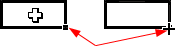
You can use the fill handle to quickly enter data series. The fill handle is the small black square in the lower-right corner of a selected cell or range. When you hover the mouse pointer over the fill handle, the pointer changes from  to
to  , and you can then drag to fill.
The following exercise demonstrates using a built-in list and pattern recognition. The table that follows provides examples for further experimentation.
Task 3.3 Built-in list
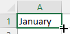
Create a new worksheet.
Select cell A1 and type “January”.
Select cell A1 again. Position the mouse over the fill handle of cell A1. Press and hold the left mouse button, drag down to cell A12, and then release the mouse button.
 .
.
The range A1:A12 is filled with the months of the year. You can start with any month, and the sequence will repeat if you continue dragging.
Pattern recognition
Select cell B1 and type the number 1.
Select cell B2 and type the number 2.
Select the range B1:B2 and drag the fill handle down several cells.
 .
.
The range is filled with the numbers 1, 2, 3, 4, 5, and so on.
Table 3.1 shows examples for you to experiment with.
| Starting values | Auto fill series |
|---|---|
| 1, 3 | 5, 7, 9, 11, … |
| 2, 4 | 6, 8, 10, 12, … |
| 3, 6 | 9, 12, 15, 18, … |
| 2010, 2011 | 2012, 2013, 2014, … |
| 09:00 | 10:00, 11:00, 12:00, 13:00, … |
| Jan | Feb, Mar, … |
| Jan, Apr | Jul, Oct, Jan, Apr, … |
| Monday | Tuesday, Wednesday, … |
| Mon | Tue, Wed, … |
| Q 1 | Q 2, Q 3, Q 4, Q 5, … |
| 1e period | 2nd period, 3nd period, … |
| article 1 | article 2, article 3, article 4, … |