6 Formulas and Functions
- Types of functions and the syntax of a function.
- Entering a function manually and with the Wizard.
- Nesting of functions.
Excel has more than 300 built-in functions to perform various operations. These functions are organized into categories, such as:
- Database
- Date & Time
- Financial
- Information
- Logical
- Statistical
- Engineering
- Text
- Math & Trig
- Lookup & Reference
Categories can be helpful when searching for a specific function. For example, to find a function that calculates loan repayments, you can look in the Financial category. Other categories include: All, Most Recently Used, and User Defined.
Most functions require you to specify the values or cell contents they should use in the calculation. These are called arguments.
All Excel functions follow the same structure (syntax), as shown in Figure 6.1.
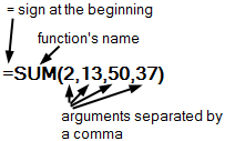
- They begin with an equal sign
=. - Followed by the function’s name.
- Then, parentheses enclose the arguments, separated by commas.
- Arguments can be numbers, text, operators, or even other functions.
The argument separator (comma or semicolon) depends on your Windows regional settings. English versions typically use a comma, while other language versions (e.g., Dutch) may use a semicolon. You can change this in the Windows Control Panel.
Function names and argument separators vary depending on the language version of Microsoft Office.
This chapter discusses some commonly used functions through practical examples.
6.1 Entering Functions
You can enter functions using the Function Wizard or manually. The best method depends on your experience level and whether you already know the function’s name and syntax. Both methods are explained below. The Function Wizard is used in the examples, but you can also enter functions manually.
6.1.1 Function Wizard
The Function Wizard is helpful for beginners and less experienced users. You can open it in two ways:
- Click the \(f_x\) Insert function button at the beginning of the formula bar.
- Go to Formulas > Insert Function (Function Library group)
The Insert Function dialog box will appear:
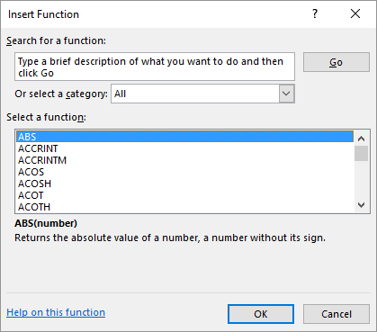
To quickly find the right function, first select a function category from the drop-down list. If you’re unsure which category to choose, select All.
Select the desired function, such as COUNTIF, and click OK. The Function Arguments dialog box for the selected function will appear.
In this dialog box, you can specify the function’s arguments. The required arguments depend on the selected function. You can type the arguments directly, or for cell addresses, you can select the cells in the worksheet using the mouse.
For detailed help on the function, click the Help on this function link.
6.1.2 Autocomplete Functions
If you are familiar with a particular function, its correct spelling, and the types of arguments it requires, you can type the function and its arguments directly into the formula bar. This is often the most efficient method.
Excel’s Autocomplete Functions feature is very useful for manual entry. When you type an = sign and the first few letters of a function in a cell or the formula bar, Excel displays a drop-down list of all valid entries that begin with those letters. Icons indicate the entry type, such as a function or cell/table reference. A screen tip also provides a brief description of each function.
Continue typing the function name to narrow the list, or use the arrow keys to select the function from the list. After selecting the desired function, press Tab to insert the function name and an opening parenthesis into the cell.
Once you insert the function and the opening parenthesis, Excel displays another screen tip showing the function’s arguments. The argument in bold is the one you are currently entering. Arguments in parentheses are optional.
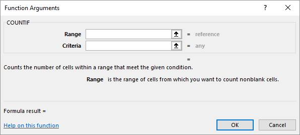
Example 6.1 Autocomplete
Figure 6.4 illustrates an example. In the first image, the letter c has been entered. The list box displays all functions that start with c.
In the second image, ou has been added. The list now shows all entries that start with cou. A screen tip displays information for the selected function, COUNTIF.
Pressing Tab results in the third image. This function requires two arguments.
6.2 Autosum
Since addition is a frequently used operation, Excel provides the Autosum button on the ribbon in the Editing group (Home tab) for quick entry. Using the Function Wizard for addition often requires multiple mouse clicks, so Autosum can save time.

The arrow next to the Autosum button provides a drop-down list with quick access to the Average, Count Numbers, Max, and Min functions.
Task 6.1
Start with a new worksheet.
Enter the following numbers in cells A1:A6: 120, 121, 122, 123, 124, and 125.
Select cell A7, and then click the Autosum button.
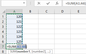
Excel places a selection border around the cells that it assumes you want to sum. If this is not the correct range, use the mouse to select the desired area.
Confirm the selection by doing one of the following:
- Click the Autosum button again.
- Click the Enter button,
 , in the formula bar.
 - Press the Enter key on the keyboard.
Cell A7 will display the result 735. The formula in cell A7 is =SUM(A1:A6), which is shorter and clearer than =A1+A2+A3+A4+A5+A6.
6.3 Mathematical Functions
The mathematical functions category is quite extensive. In addition to the common SUM function for adding numbers, this category includes functions for various calculations, such as exponentiation, square roots, PI, logarithms, and trigonometry.
Functions for rounding numbers are common. Excel provides thirteen rounding functions, which can make it challenging to choose the appropriate function. For example, the ROUND function rounds a number up or down to a specified number of decimal places. Other functions round to the nearest multiple of a given number or to the nearest integer.
Task 6.2 File: Rounding.xlsx
Figure 6.6 shows the results of several rounding functions. Column C displays the formulas used in column B.
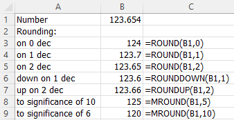
Open the file.
Enter the appropriate formulas in cells B3:B9 using the Function Wizard.
6.4 Statistical Functions
The statistical category contains functions for statistical analysis, such as average, count, minimum, and maximum.
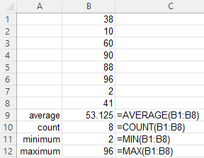
Task 6.3 File: Statistics.xlsx
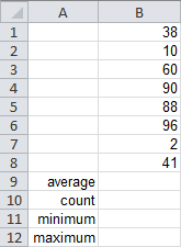
Open the file.
In cells B9 to B12, perform the calculations using the functions from the table below. These functions are in the Statistical category.
- B9:
AVERAGE - B10:
COUNT - B11:
MIN - B12:
MAX
- B9:
The argument is always the range B1:B8. Although you can type this range in the Function Arguments dialog box, it’s more convenient to place the cursor in the box for the first argument and then select the range B1:B8 in the worksheet with the mouse.
6.5 Date and Time Functions
The Date and Time category provides functions for working with dates and times. Because Excel stores dates and times as numbers internally, you can perform calculations with them. The American date format is Month/Day/Year.
Task 6.4 File: Date.xlsx
- Open the file.
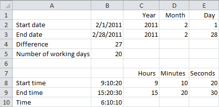
First, extract the year, month, and day values from the start and end dates.
Use the
YEAR,MONTHandDAYfunctions to determine the values in cells C2, D2, and E2. The argument for these functions is cell B2.Select C2:E2 and drag the fill handle one row down.
Select cell B4 and enter the formula
=B3-B2. The result is 27.
The NETWORKDAYS function calculates the number of workdays between a start date and an end date. It excludes weekends and dates specified as holidays. You can use an optional argument to specify holidays.
Select cell B5, and calculate the number of workdays. Enter the cell addresses for the start and end dates; leave the holidays box empty.
Similarly, calculate the hours, minutes, and seconds from the start and end dates using the
HOUR,MINUTE, andSECONDfunctions.Calculate the time difference in B10 using a formula.
Subtract the start time from the end time.
6.6 Logical Function IF
Logical functions work with the results TRUE or FALSE. The most common logical function is the IF() function. In simple terms, this function works as follows:
=IF(condition, value_ if_true, value_if_false)
The condition is a logical test that evaluates to either TRUE or FALSE.
For more than one condition, you can nest IF() functions. However, nested IF() functions can become complex and difficult to read. Consider using the logical functions AND(), OR(), and NOT() instead.
Task 6.5 Figure 6.9 shows marks with their corresponding pass/fail status. The status is determined automatically based on the mark. A mark less than 5.5 is considered failing.
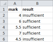
Start a new worksheet and enter the numbers shown in Figure 6.9.
Select cell B2 and use the Insert Function to insert the
IFfunction.Complete the dialog box as shown in Figure 6.10. You can type the quotation marks around the text, but it is not required as Excel will add them automatically.
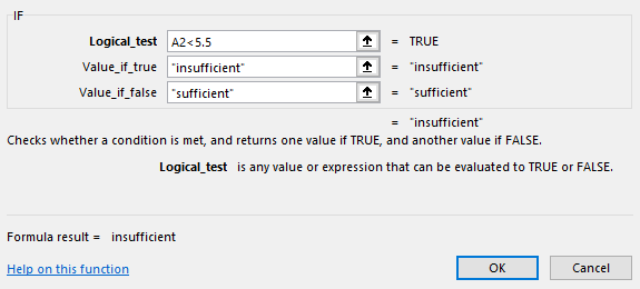
Click OK.
Select cell B2 and drag the fill handle to B6.
6.7 Text Functions
This section demonstrates splitting text into different parts using four text functions.
Excel includes functions for manipulating text. For example, you can determine the length of a text string or extract specific parts of a string.
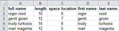
Figure 6.11 shows full names in column A. The goal is to extract the first and last names into separate columns. In this example, the first and last names are separated by a space, which can be used as a delimiter. To extract the names, you need to find the position of the space and know the total length of the text. The text before the space is the first name, and the text after the space is the last name.
The results are shown in columns B to E in Figure 6.11. This exercise is divided into four parts, each using a different function.
6.7.1 LEN
The LEN function determines the length of a text string.
Task 6.6 File: Names.xlsx
Open the file.
Select cell B2 and insert the
LENfunction with cell A2 as argument.Drag the fill handle in B2 down to B5.
Column B now displays the length of the full names.
6.7.2 SEARCH
The SEARCH function finds the starting position of a specific character (or string) within a text. In this case, it finds the position of the space.
Task 6.7
- Select cell C2 and click the Insert Function button on the formula bar.
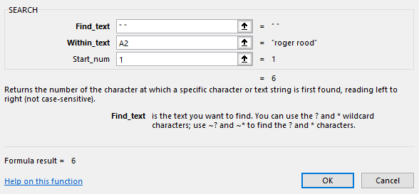
Click OK.
Drag the fill handle in C2 down to C5.
Column C now displays the position of the first space in each name.
6.7.3 LEFT
The LEFT function extracts a specified number of characters from the beginning of a text string. In this example, it extracts the first name.
Task 6.8
- Select cell D2, insert the
LEFTfunction, and enter the arguments as shown in Figure 6.13.
In the Num-chars box, specify the length of the text to extract. This is one less than the position of the space, which is found in cell C2.
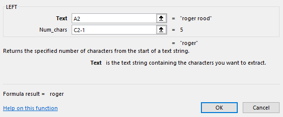
Click OK.
Drag the fill handle in D2 down to D5.
Column D now displays the first names.
6.7.4 RIGHT
The RIGHT function extracts a specified number of characters from the end of a text string. In this example, it extracts the last name.
Task 6.9
- Select cell E2, insert the
RIGHTfunction, and enter the arguments as shown in Figure 6.14.
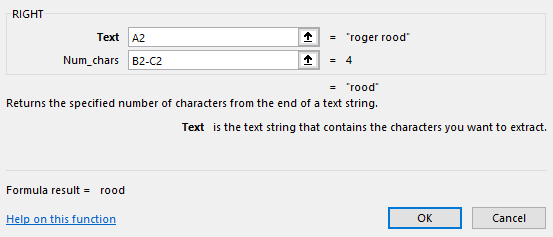
In the Num_chars box, enter the length of the right-hand portion. This is counted from the end of the text. In this example, the length of the right-hand portion is equal to the total length of the text (the value in B2) minus the position of the space (the value in C2).
Click OK.
Drag the fill handle in E2 down to E5.
Column E now displays the last names.
6.8 Nested Functions
A nested function is a function within another function, where one function acts as an argument for the other. For example:
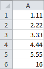
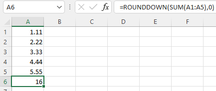
=ROUNDDOWN(SUM(A1:A5),0)
The following exercise uses a nested function.
Task 6.10
- Start a new worksheet, and enter the data shown in Figure 6.15.
- Select cell A6, and insert the
ROUNDDOWNfunction (from the Math & Trig category).
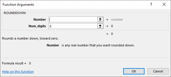
In the function’s arguments dialog box, the cursor will be in the Number field. It’s often helpful to specify the number of decimal places first, and then define the range of numbers.
- Place the cursor in the Num_digits field, enter
0, Then, move the cursor back to the Number field.
- Click the arrow in the name box on the worksheet.
A drop-down list appears, showing the names of the most recently used functions. At the bottom of this list, you’ll see More Functions.
Click on More Functions. The familiar Insert Function dialog box will appear.
In the Math & Trig category, select the
SUMfunction and click OK.
The Function Arguments dialog box appears. The Number1 argument already contains the value A1:A5.
- Click OK.
The result appears in cell A6, and the formula used is displayed in the formula bar.
If you hadn’t entered the number of decimals after step 3, you would have received a warning during nesting indicating that too few arguments were entered. You would have had to correct this manually in the formula.
A faster way to work is to type the formula directly into the formula bar. As you type, you’ll receive assistance with entering the formula. However, this method requires you to know the names of the functions you want to use.
6.9 COUNTIF
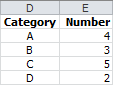
The COUNTIF function is very useful for creating frequency tables. Figure 6.18 shows a list of camping sites and their categories. Column E will contain the number of campsites in each category.
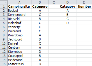
Task 6.11 File: Campsites.xlsx
Open the file.
Select cell E2, insert the
COUNTIFfunction, and specify the arguments as shown in Figure 6.19.
Specifying the entire column B as the range allows you to add new rows of data to the bottom without needing to change the formulas.
Click OK.
Select cell E2 and drag the fill handle down to E5.
6.10 SUMIF
The SUMIF function allows you to add numbers based on specific conditions. The spreadsheet contains a list of yields for different coffee types, organized by month and region. You’ll use it to determine the total yields per region.
Task 6.12 File: Coffee.xlsx
Open the file.
Select cell H2, insert the
SUMIFfunction, and enter the arguments as shown in Figure 6.20.
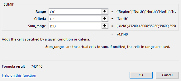
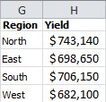
Click OK. The total yield for North region, 743140, now appears in cell H2.
Select cell H2 and drag down the fill handle to H5.
Format the numbers in H2:H5 as currency.
In this case, a pivot table would be an easier way to create this summary.
6.11 Calculating Annuities
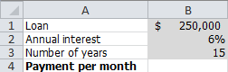
There are several ways to calculate loan repayments. This example calculates the monthly repayment amount for a $250,000 loan with a 6% fixed annual interest rate over 15 years, using an annuity. We’ll use the Excel function PMT, which calculates the payment for a loan based on constant periodic payments and a constant interest rate.
Task 6.13 File: Repayment.xlsx
Open the file and format the cells as shown in Figure 6.21.
Select cell B4, insert the
PMTfunction (from the Financial category) and enter the arguments as shown in Figure 6.22.
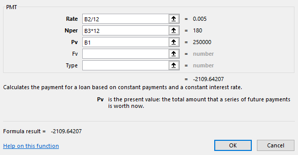
Because the period in this example is in months rather than years, the annual interest rate must be divided by 12, and the number of years must be multiplied by 12.
- Click OK.
The result -2109.64 appears. Because this is an amount to be paid (a debt), Excel displays it as a negative number, shown in red font and with a minus sign.
- To change this to a positive number, insert a minus sign after the
=sign in the formula. The formula will then be=-PMT(B2/12,B3*12,B1).
6.12 Calculating Number of Periods
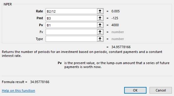
Suppose you take out a personal loan of €4,000 and agree to pay a monthly amount of €125. Calculate the number of months it will take to repay the loan at a 6% fixed annual interest rate. For this calculation, we’ll use the Excel function NPER. This function calculates the number of periods for an investment based on periodic, constant payments and a constant interest rate.
Payments are entered as negative numbers.
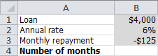
Task 6.14 File: Payment_Periods.xlsx
Open the file.
Select cell B4, insert the
NPERfunction (from the Financial category) and enter the arguments as shown in Figure 6.24.
NPER function.
Because the period is in months and not years, the annual interest rate has been divided by 12.
- Click OK. The result 34,95778166 appears, indicating almost 35 months.
6.13 Vertical Lookup
The VLOOKUP function searches for a specified value in the first column of a list (table) and returns the corresponding value from another column.
Syntax: VLOOKUP(lookup-value, table-array, col-index-num, [range-lookup])
The last argument is optional and can be set to FALSE or TRUE.
- FALSE: Searches for an exact match with the specified lookup value.
- TRUE: Returns the closest match below the lookup value if an exact match is not found.
In most cases, it’s best to search for an exact match; otherwise, you might get incorrect results. If you allow an approximation, the leftmost column of the table array must be in ascending order.
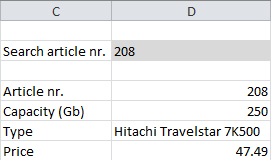
Figure 6.25 shows an overview of hard drives, with the article number in the first column. Using the VLOOKUP function, you can find the capacity, type, and price of an item by entering its article number.
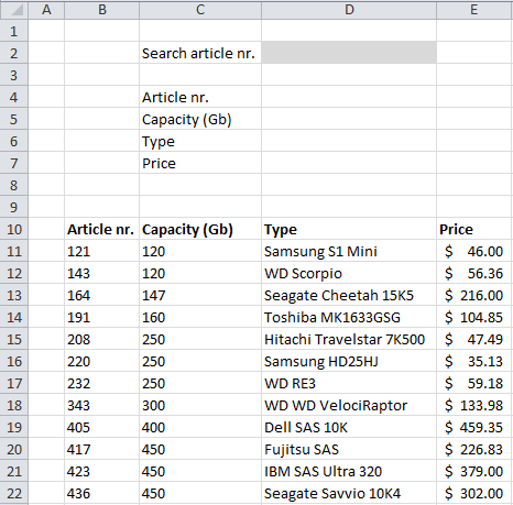
Cell D2 is the input cell for the article number you want to search for. Cells D4:D7 will contain the lookup formulas.
Task 6.15 File: Harddisks.xlsx
Open the file.
Select cell D4 and enter the formula:
=VLOOKUP($D$2,$B$11:$E$22,1,FALSE).
The error #N/A appears in the cell because there is no search value in cell D2 yet.
Enter the value
208in cell D2. Now, 208 (the article number) appears in cell D4.Enter the correct lookup formulas in the other three cells:
D5:
=VLOOKUP($D$2,$B$11:$E$22,2,FALSE).D6:
=VLOOKUP($D$2,$B$11:$E$22,3,FALSE).D7:
=VLOOKUP($D$2,$B$11:$E$22,4,FALSE).
6.14 Horizontal Lookup
The HLOOKUP function searches for a specified value in the first row of a list (table) and returns the corresponding value from another row.
Syntax: VLOOKUP(lookup-value, table-array, row-index-num, [range-lookup])
The last argument is optional and can be set to FALSE or TRUE:
- FALSE: Searches for an exact match with the specified lookup value.
- TRUE: Returns the closest match to the left of the lookup value if an exact match is not found.
It’s generally best to search for an exact match; otherwise, you might get incorrect results. If you allow an approximation, the top row of the table array must be in ascending order.
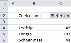
Figure 6.27 shows an overview of shoe sizes for several people, with their names in the first row. You can use the HLOOKUP function to find the corresponding age, height, and shoe size when you enter a name.
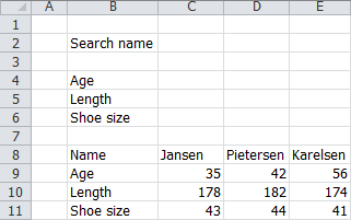
Cell C2 is the input cell for the name to be searched. Cells C4:C6 will contain the lookup formulas.
Task 6.16 File: Shoe_Sizes.xlsx
Open the file.
Select cell C4 and enter the formula
=HLOOKUP($C$2,$C$8:$E$11,2,FALSE).
The error #N/A appears in the cell because there is no search value in cell C2 yet.
Enter the value
Pietersenin cell C2. Now, 42 (the age) appears in cell C4.Enter the correct lookup formulas in the other two cells:
C5:
=HLOOKUP($C$2,$C$8:$E$11;3,FALSE).C6:
=HLOOKUP($C$2,$C$8:$E$11;4,FALSE).
6.15 Exercises
Exercise 6.1 Computer Company Results (form001)
File: Form001.xlsx
The following table shows the results of a computer company for 2010. The company’s goal is to achieve a gross profit per product of more than $5,000 and a realized margin of more than 15%. The operating result is considered “good” only if both targets are met; otherwise, it’s considered “bad.”
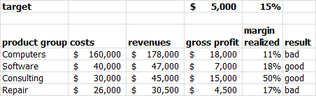
Create this model in a worksheet. Use formulas to calculate the gross profit, the margin, and the result. The result should update automatically if the gross profit and margin targets are changed.
Exercise 6.2 Lookup Article Details (form002)
File: Form002.xlsx
A computer store has the following article information in a table: article number, name, and price. To quickly find data for a specific article, the article number can be entered in a cell. The corresponding name and price are then automatically looked up in the table.
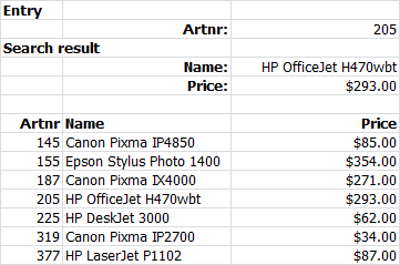
Enter the data in a worksheet and use formulas (VLOOKUP) to retrieve the search results.
Exercise 6.3 Calculating with Dates (form003)
File: Form003.xlsx
In the following table, you can enter your date of birth and the retirement age (67 years). The date you reach retirement, the current date, and the number of days until your retirement date should be calculated using formulas.
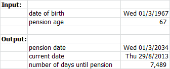
Create this model in a worksheet and use formulas to calculate the output results.
Used functions:
DATE,YEAR,MONTH,DAY,TODAY.You can format a date like “Wed 01/3/1967” using the cell’s number format. Go to Home tab > Category Custom (Number group), or right-click the cell and select Format Cells. In the Type box, enter the desired format. The format used in the example is “ddd dd/m/yyyy”. Try other formats like “dddd dd/mmm/yy” to understand how the formatting works.
In Excel, a date is actually just a number, which you can use in calculations. To find the time difference between two dates, subtract them.
Exercise 6.4 Determining Commission (form004)
File: Form004.xlsx
A company with three salespeople has a target of $150,000 in sales per year for each person. If a salesperson reaches that amount, their commission is 6.25% of their sales. If not, their commission is only 5.5%. The following figure shows a model for calculating the commission for each salesperson.
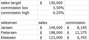
Create this model in a worksheet and use formulas for the calculation of the commissions.
Exercise 6.5 Birth Dates (form005)
File: Form005.xlsx
A mother-child center at a hospital wants a daily overview of babies born too early, on time, and too late. For babies born too early or too late, they also want to know how many days early or late. For babies who are yet to be born, they want to know how many days overdue they are.
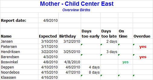
Create this model in a worksheet. Also, create a similar layout.
The last four columns depend on one or more conditions, so you’ll need to use the
IFfunction.For two conditions, you can nest a second
IFfunction within the firstIFfunction. Alternatively, you can use theANDfunction within theIFfunction.A birth date is considered “too early” if it’s before the expected date.
In Excel, a date is simply a number, so you can compare dates using operators like <, >,
Exercise 6.6 VAT Return (form006)
File: Form006.xlsx
A company buys goods from suppliers and pays sales tax (VAT) to those suppliers. The company then sells the goods to customers, who pay VAT to the company. Every quarter, the company must submit a tax declaration. The difference between the VAT received (from sales) and the VAT paid (to suppliers) must be paid to the tax authority. If this difference is negative, the company receives a refund. Small businesses may be eligible for a reduction in VAT through the Small Businesses Regulation (SBR). This regulation is outlined in the following table.
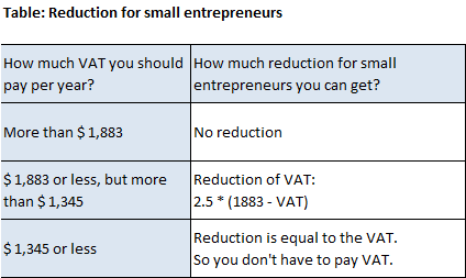
Create a model with cells for entering the total sales and prepaid VAT, and cells for the constants (the thresholds and VAT percentage). Calculate the initial VAT to be paid, the reduction, and the final amount to be paid or received in other cells. Use a single VAT rate of 21%. The final amount should automatically be labeled as a payment or a receipt. All amounts must be formatted as whole euros.
Thoroughly test the model with all possible scenarios.
Exercise 6.7 Ticket Price (form007)
File: Form007.xlsx
The following table shows the ticket prices for a sports game. There are two categories: children and adults. There’s also a cell for entering the age (in whole years). After entering the age, the ticket price is automatically calculated.
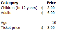
Create this model in a worksheet. Use an IF function for the price calculation. Test the solution with different ages.
Exercise 6.8 Property Tax (form008)
File: Form008.xlsx
The property tax has two parts: an owner’s portion and a user’s portion. If the owner occupies the property themselves, they must pay both portions. The rate for both portions depends on the assessed value according to the WOZ Act. The property tax for 2010 in a certain community is 0.1064% of the WOZ value for the owner and 0.1224% for the user.
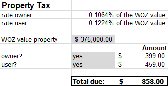
Create this model in a worksheet. The calculated values for the owner and user depend on the answers “yes” or “no” to both questions.
Exercise 6.9 Savings Deposit (form009)
File: Form009.xlsx
An amount of $20,000 will be placed in a savings deposit for one year at an interest rate of 2.75%. Create a calculation model that calculates both the interest and the total amount after one year.
Interest = $ 550.00 and Amount = $ 20,550.00
Exercise 6.10 Joule’s Law (form010)
File: Form010.xlsx
The amount of heat generated by an electric current flowing through a conductor can be calculated using Joule’s law: \(Q = 0.24 * i^2 * R * t\)
Where:
Q: The amount of heat (cal)i: Current (ampere)R: Resistance (ohm)t: Time (sec)
Create a model in a worksheet where the current, resistance, and time can be entered, and the amount of heat is calculated from the entered data.
Exercise 6.11 Investment Bond (form011)
A government bond with a maturity of 5 years pays an annual interest rate of 3.5%. Suppose you want to have $300,000 after 5 years; how much do you need to invest in this bond? Use Excel’s present value function (PV) to calculate the answer.
$ 252,592
Exercise 6.12 Multiplication Table (form012)
First, create the following table:
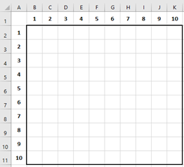
Then, enter a formula in cell B2 that you can copy down and to the right to fill the rest of the table, so that the value in each cell is the product of the number to the left of the row and the number above the column.
You’ll need a combination of absolute and relative addressing in your formula.
Exercise 6.13 Price of Olive Oil (form013)
Olive oil can be purchased in 5-liter cans. The price depends on the number of cans:
- $45 per can for the first 20 cans
- $40 for any can beyond 20
Create a spreadsheet model where you can enter the total number of cans, and the total price is calculated. Use separate cells for the price per can and the 20-can limit. Name all the cells appropriately.