15 Solver
- Learn how to activate the Solver add-in.
- Understand the applications of Solver.
- Learn how to set up a calculation model for Solver.
- Understand how to add constraints in Solver.
- Discover tips for using Solver effectively.
Solver is an Excel add-in used for optimization calculations. In such calculations, you aim to find an optimal value (usually a minimum or maximum, but sometimes a specific value) for a formula in a particular cell.
- Objective Cell (Target Cell)
-
This is the cell containing the formula for which you want to find an optimal outcome.
- Variable Cells (Changing Cells, Decision Variables)
-
These are the cells whose values determine the outcome of the formula in the objective cell. Changing these values alters the formula’s result.
- Constraints (Restrictions, Preconditions)
-
These are limitations or conditions that apply to the variable cells. Variable cells often cannot take on any possible value and are bound by these limits.
Solver offers more extensive “What-If” analysis capabilities than Goal Seek and is much more versatile. Solver adjusts the values in the changing cells, within the defined constraints, to find the optimal solution for the objective cell.
15.1 Enabling Solver
Solver is an add-in and is not activated by default in Excel’s menu. If Solver is not present on the Data tab of the ribbon, it must be activated first. This is a one-time action.
First, check if Solver is available on the ribbon. If it is, you can skip this task. Select the Data tab and check if the AnalyzeAnalyze group exists and if Solver is present within it.
Task 15.1
Choose File > Options > Add-Ins. A list of Microsoft Office Add-ins will be displayed.
In the Manage box at the bottom, select Excel Add-ins.

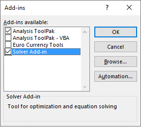
Click on Go…. A list of available Add-ins will be displayed.
Select the checkbox for Solver Add-in and click on OK.
- Repeat the check above to ensure Solver is now visible.
15.2 Defining an Optimization Model
To perform an optimization calculation, you must first set up a suitable calculation model. This is often more challenging than using Solver itself. The process of creating such a model will be explained using the WeatherLeather case study.
15.2.1 Case Description
WeatherLeather, a manufacturer of high-end leather jackets, has designed two styles for the new season: a long jacket and a short jacket. Manufacturing a short jacket requires 1 hour in the cutting department and 3 hours in the sewing department. A long jacket requires 2 hours and 4 hours, respectively. Labor hour availability is limited: the cutting department has 32 hours per week, and the sewing department has 84 hours per week. Market demand for long leather jackets is also limited; no more than 12 long leather jackets can be sold per week. For short jackets, all manufactured jackets can be sold. Production is not to stock. The profit for a short jacket is $90, and for a long jacket, it is $144.
The question is: How many jackets of each type should be made per week to achieve the highest possible profit?
15.2.2 Understanding the Problem
This step might seem obvious, but it’s crucial to fully understand the problem before formulating the objective cell, variable cells, and constraints. Misunderstanding the problem can lead to an incorrect model. In this example, the problem is relatively straightforward:
How many short and long jackets should be produced weekly to maximize profit, given that no more than 32 hours of cutting time and 84 hours of sewing time are available, and the market for long jackets is limited to 12 per week?
15.2.3 Decision Variables
Identify the decision variables. These are the variables for which you need to determine values that yield the optimal result. In the Excel model, these correspond to the variable cells. In this example, there are two decision variables, conveniently denoted by letters:
- \(S\) = number of short jackets per week
- \(L\) = number of long jackets per week
15.2.4 Objective Function
You must establish a formula that represents the value you want to optimize. The decision variables are included in this formula. In this example, the objective function is the weekly profit, which depends on the number of short jackets (\(S\)) and long jackets (\(L\)) produced:
\(Profit = 90 \times S + 144 \times L\) (This function should be maximized.)
In more complex models, it can sometimes be challenging to formulate the problem with a single objective function. It may also happen that the decision variables are not directly in the objective function. In such cases, the objective function contains variables whose values depend on the decision variables.
15.2.5 Constraints
Usually, there are restrictions on the values that the decision variables can take. These restrictions must be identified and formulated.
In this example, three constraints come directly from the case description: the limited capacities of the cutting and sewing departments, and the market demand for long jackets.
Additionally, there are often general constraints related to the nature of the decision variables. In this example, the two decision variables (the number of jackets produced) must be non-negative integers.
This leads to the following constraints:
- Cutting time constraint per week: \(1 \times S + 2 \times L \le 32\)
- Sewing time constraint per week: \(3 \times S + 4 \times L \le 84\)
- Market demand constraint for long jackets: \(L \le 12\)
- Non-negativity constraints: \(S \ge 0\) and \(L \ge 0\)
- Integer constraints: \(S = integer\) and \(L = integer\)
15.2.6 Model in Excel
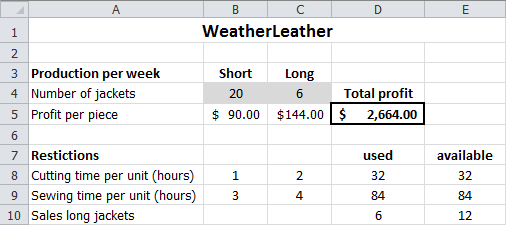
Now it’s time to build the model in Excel and solve the problem using Solver. One possible layout is shown in Figure 15.4.
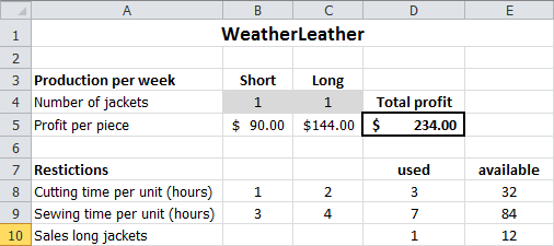
There isn’t one single correct way to build this model in Excel, but some guidelines can help. These guidelines are discussed based on Figure 15.4. You can build the model yourself using these guidelines and the figure, or use the provided file WeatherLeather.xlsx.
15.2.7 Guidelines for a Solver Model in Excel
Organize the data logically and clearly. Add sufficient explanatory text near cells containing numbers and formulas. Models are often used in reports later, so it must be clear what everything represents. Highlight the cells for decision variables (e.g., B4 and C4) and the objective function (e.g., D5) so they are easily recognizable. Place constraints in a separate section.
Put each decision variable in a separate cell and assign it an initial value. In the example, the number of short and long jackets produced are in cells B4 and C4, respectively. An initial value of 1 is used for both, allowing for easy verification of formulas.
Create a formula for the objective cell. In D5, the formula is
=B5*B4+C5*C4.Create a formula in a separate cell for the left-hand side of each constraint. In an adjacent cell, place the limit (right-hand side) of the constraint.
| Cell | Formula | Explanation |
|---|---|---|
| D8 | =B8*B4+C8*C4 |
Total cutting time calculation |
| D9 | =B9*B4+C9*C4 |
Total sewing time calculation |
| D10 | =C4 |
Number of long jackets produced |
15.2.8 Solver Constraints
The dialog box in Solver used to add constraints is shown in Figure 15.5.
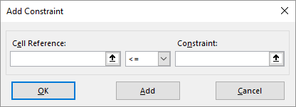
Every constraint in Solver consists of three parts: a cell reference, a relationship operator, and a constraint value.
- Cell Reference
-
he cell address or name of the cell range whose values you want to constrain. You can use a single cell or a contiguous cell range, but not multiple disconnected ranges in a single constraint entry.
- Relationship
-
Possible operators:
<=,=,>=,int,bin, ordif. -
int: The values in the cell reference(s) must be integers (within a certain tolerance defined by the “Constraint Precision” in Solver options).
-
bin: The values in the cell reference(s) must be binary (either 0 or 1). This can be used for “yes/no” decisions.
-
dif: The values in the specified cell references must all be different from each other.
- Constraint
-
A number, a cell reference (or name), or a formula that the cell reference must adhere to based on the relationship.
15.3 Implementing the Model
In the WeatherLeather case, the profit must be maximized.
Task 15.2 File: WeatherLeather.xlsx
Open the file.
Select the objective cell, D5.
Choose tab Data > Solver (Analyze group). The Solver Parameters dialog box will appear.
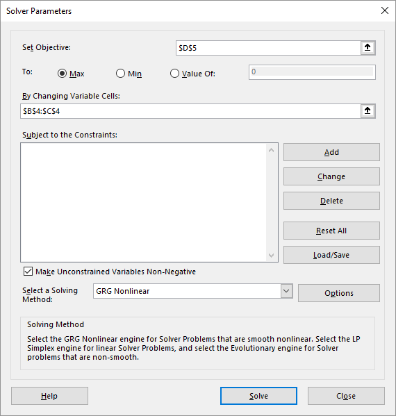
Verify the following:
- Set Objective:
$D$5 - To:
Max
- Set Objective:
Click in the By Changing Variable Cells box and select the cell range B4:C4 in the worksheet. Excel will convert this to
$B$4:$C$4.In the Subject to the Constraints section, click Add. The Add constraint dialog box will appear (see Figure 15.5)
Add the constraint
D8 <= E8(Cell Reference: D8, Relationship: <=, Constraint: E8) and click OK.
The Solver Parameters dialog box will reappear, showing the first constraint as $D$8 <= $E$8.
Click Add again.
Add the constraint
D9 <= E9and this time click Add (instead of OK).
The empty Add Constraint dialog box will remain displayed. You won’t see the second constraint added to the main Solver Parameters dialog box yet, but it has been registered.
By clicking Add instead of OK after entering a constraint, you can add multiple constraints more efficiently without repeatedly returning to the Solver Parameters dialog box.
Add the constraint
D10 <= E10and click Add.Add the constraint
B4:C4 >= 0and click Add.Addt the constraint
B4:C4 = integer(selectintfrom the dropdown).All constraints have now been added. Click OK in the Add Constraint dialog box.
The Solver Parameters dialog box will now show all specified constraints.
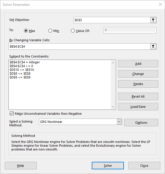
- Click Solve. After a short time, the Solver Results dialog box will appear.
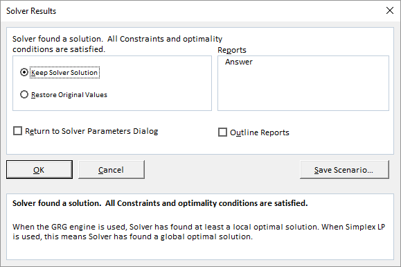
- Select Keep Solver Solution (this is usually the default). In the Reports section, select Answer and then click OK.
The solution found by Solver will now be displayed in your worksheet.
A new worksheet named Answer Report … will also be created.
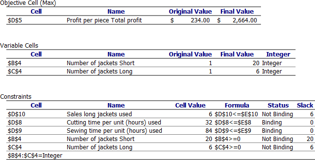
The names used in the Answer Report are not always perfectly descriptive. Excel attempts to derive these names from text in adjacent cells in your model. To ensure clear names in the report, it’s highly recommended to define meaningful names for the relevant cells in your worksheet (using the Name Box or Name Manager) before running Solver.
In the Constraints section of the Answer Report, the Status column indicates which constraints are Binding. A binding constraint means its limit has been reached, and there is no slack. In this example, you can see that all available cutting time and sewing time are used. For the long jackets, the market demand limit is not reached; there is a slack of 6 (meaning 6 more could potentially be sold if other constraints allowed).
The WeatherLeather problem is now solved. A maximum profit of $2,664 per week can be achieved by producing 20 short jackets and 6 long jackets.
15.4 No Solution Found. What Now?
Frequently, Solver reports that no feasible solution could be found:
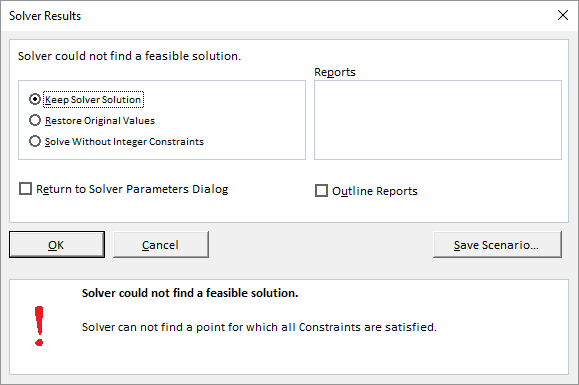
There are two main possibilities:
- No solution actually exists for the problem as formulated.
- A solution does exist, but Solver was unable to find it.
In most cases, it’s not immediately certain which situation applies. Here are a few guidelines to investigate if Solver can find a solution:
15.4.1 Changing Initial Values of Variable Cells
Solver’s ability to find a solution can depend on the initial values of the variable cells. Experimenting with different starting values can sometimes help Solver find a solution, especially for non-linear problems.
15.4.2 Changing Solver Options
Finding a solution also depends on how Solver operates. The search for a solution is an iterative process (repeated recalculations until a specific condition is met). Solver has several settings for this iteration process. Clicking the Options button in the Solver Parameters dialog box opens a window for changing these settings.
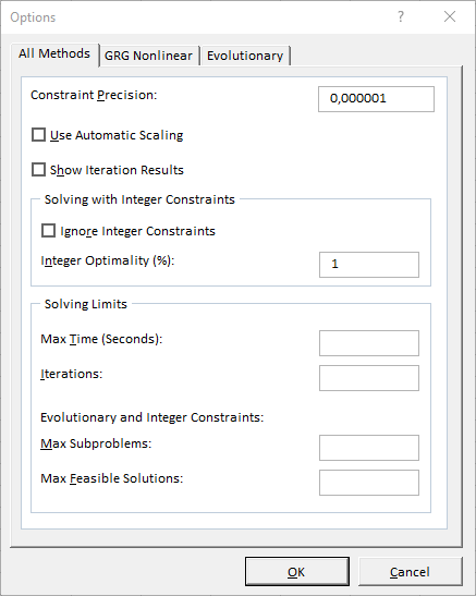
This dialog box offers extensive control over the solution process. Specifications for certain problem types can be saved as a model and reloaded. Some key settings are:
| Option | Explanation |
|---|---|
| Max Time | The maximum time Solver is allowed to spend on the solution process. |
| Iterations | The maximum number of iterations (recalculations) Solver will perform. |
| Constraint Precision | The degree of precision required for a constraint to be considered satisfied. A smaller number means higher precision. (Note: The original table had ‘Precision’ and ‘Constraint Precision’ - this is a common point of confusion. ‘Constraint Precision’ is the key one for how closely constraints must be met). |
| Integer Optimality (%) | The maximum percentage difference from the true optimal integer solution that is acceptable. A value of 0 means Solver must find the exact optimal. A small percentage (e.g., 1%) can speed up complex integer problems. (Original table had ‘Tolerance’ which is related but ‘Integer Optimality’ is the standard term here). |
| Assume Linear Model | Check this if all relationships in your model are linear. This can speed up the solution process. Using it with non-linear models may prevent Solver from finding a solution or lead to an incorrect one. Show Iteration Results Select this to pause Solver after each iteration and see the trial solution. Not typically used unless debugging a difficult problem. |
Additional information:
Visit the support site of Frontline Systems, the developers of Solver, for the most comprehensive information.
15.5 Exercises
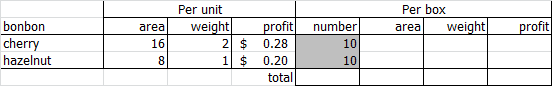
Exercise 15.1 Bonbon Box Assortment (solv001)
A renowned bonbon manufacturer wants to offer an assortment box with two types of chocolates (cherry bonbons and hazelnut chocolates) to maximize profit. The following information is known:
- A cherry bonbon takes up 16 cm2 of space, and a hazelnut bonbon takes up 8 cm2. The bonbons are separated by paper. At least 320 cm2 of the box must be covered with bonbons.
- A cherry bonbon weighs 2 grams, and a hazelnut bonbon weighs 1 gram. Market research indicates the ideal weight of the box’s contents is between 40 grams and 60 grams (inclusive).
- Market research also revealed that the box must contain at least 35 bonbons in total, with at least 10 of them being cherry bonbons.
- The profit on a cherry bonbon is $0.28, and on a hazelnut bonbon is $0.20 .
- What are the decision variables?
- What is the objective function?
- What are the constraints?
- Build the model in Excel using the guidelines from this chapter. An example layout is shown below. Formulas need to be placed in the empty cells for calculated values (like total space, total weight, total bonbons, total profit). Both decision variables (number of each bonbon type) have an initial value of 10. These starting values allow you to easily check if your formulas are correct.
- Enter the model into Solver and determine the optimal number of each bonbon type for the box.
- Decision variables:
- C = number of cherry bonbons per box
- H = number of hazelnut bonbons per box
- Objective function (Maximize Profit P):
P = 0,28*C + 0,20*H - Constraints:
- Cherry bonbons per box quantity:
C \>= 10 - Total bonbons per boxquantity:
C + H >= 35 - Minimum box weight::
2*C + 1*H >= 40 - Maximum box weight:
2*C + 1*H <= 60 - Minimum bonbon area:
16*C + 8*H >= 320 - Integer constraint:
C, Hmust be integers - Non-negativity (implied by other constraints but good practice):
C >= 0 , H >= 0
- Cherry bonbons per box quantity:
Optimal content: 10 cherry chocolates, 40 hazelnut chocolates. Profit per box: $10.80. All constraints are met.
Exercise 15.2 Supermarket Branch Expansion (solv002)
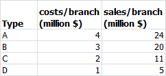
A supermarket chain plans to open new branches with a maximum investment of $14 million. The chain is considering four types of shops: A, B, C, and D. The following figure shows the setup costs for each store type and their expected sales in the next financial year.
All newly built branches can be operational for the next financial year. Potential locations are comparable in terms of population. The executive board wants to maximize the total expected sales from the new branches in the next financial year. How many branches of each type should be built?
- What are the decision variables?
- What is the objective function?
- What are the constraints?
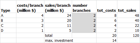
- Build the model in Excel. An example layout is provided below. Formulas are needed for calculated values (total investment, total sales). Initial values for the number of each store type are set to 2 for formula checking.
- Enter the model into Solver to determine the optimal number of branches of each type and the expected total sales.
- Decision variables:
- A = Number of Type A branches
- B = Number of Type B branches
- C = Number of Type C branches
- D = Number of Type D branches.
- Objective function (Maximize total sales S):
S = 24*A + 20*B + 11*C + 5*D - Constraints:
- Maximum investment:
4*A + 3*B + 2*C + 1*D <= 14 - Integer constraint:
A, B, C, Dmust be integers - Non-negativity:
A >= 0 , B >= 0 , C >= 0 , D >= 0
- Maximum investment:
Optimal number of branches: Type A = 0, Type B = 4, Type C = 1, Type D = 0. Total expected sales: $91.
Exercise 15.3 Running Shoe Production (solv003)
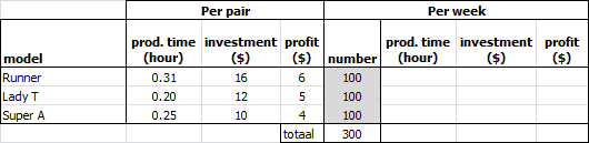
A company in Hong Kong manufactures American running shoes. The company produces three models: Runner, Lady T, and Super A, and wants to maximize profit.
- Manufacturing 1 pair: Runner requires 0.31 hours, Lady T requires 0.20 hours, and Super A requires 0.25 hours. The maximum number of production hours is 150 per week.
- Capital investment per pair: Runner $16, Lady T $12, and Super A $10. A total of $8,000 per week is available for capital investment.
- Due to limited machine capacity, weekly production is limited to: 300 pairs of Runner, 400 pairs of Lady T, and 400 pairs of Super A.
- Profit per pair: Runner $6, Lady T $5, and Super A $4.
Calculate the optimal production numbers and the maximum profit per week using Solver.
- What are the decision variables?
- What is the objective function?
- What are the constraints?
- Build the model in Excel. An example layout is below. Initial values for production quantities are set to 100.
- Enter the model into Solver to determine the optimal number of each model and the maximum weekly profit.
- Decision variables:
- R = number of Runner model pairs per week
- T = number of Lady T model pairs per week
- A = number of Super A model pairs per week
- Objective function (Maximize Profit P):
P = 6*R + 5*T + 4*A - Constraints:
- Runner production limit:
R <= 300 - Lady T production limit:
T <= 400 - Super A production limit:
A <= 400 - Maximum production time:
0,31*R 0,20*T + 0,25*A <= 150 - Maximum investment:
16*R + 12*T +10*A <= 8000 - Integer constraint:
R, T, Amust be integers - Non-negativity:
R, T, A >= 0
- Runner production limit:
Optimal production: Runner = 111, Lady T = 400, Super A = 142. Maximum profit per week: $3234.
Exercise 15.4 Aluminum Ladder Production (solv004)
A manufacturer produces three types of aluminum ladders. The production process involves sewing the material, then assembling, and finally finishing. Production times and profit per ladder are listed below:
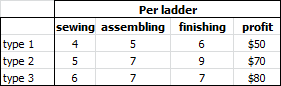
The total available production capacity per period is: 80 hours for sewing, 100 hours for assembling, and 120 hours for finishing.
Use Solver to determine how many ladders of each type should be produced to maximize profit.
Number of Type 1 = 0, Type 2 = 4, Type 3 = 10. Profit = $1,080.
Exercise 15.5 Dog Food Mix (solv005)
Two types of dog food are available: ordinary and special.
- A bag of ordinary food contains 3 units of minerals, 2 units of protein, and 3 units of fat. It costs $8.
- A bag of special food contains 8 units of minerals, 2 units of protein, and 1 unit of fat. It costs $14.
- Over a certain period, a dog must consume at least 72 units of minerals, 36 units of protein, and 36 units of fat.
Determine the quantity of each bag type to be bought to meet these nutritional requirements at minimum cost.
Number of ordinary bags = 14, special bags = 4. Minimum Cost = $168.
Exercise 15.6 Vitamins for Cattle Feeding (solv006)
A farmer uses three types of cattle feed: Type 1, Type 2, and Type 3. The nutritional composition (vitamins A, B, C in mg/kg) and cost per kg of each type are shown below:
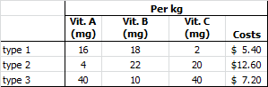
A magazine has published the minimum daily requirements (MDR) per animal for vitamins A, B, and C as 120 mg, 180 mg, and 100 mg, respectively. Furthermore, an animal cannot eat more than 7.5 kg of Type 1, 5 kg of Type 2, and 2.5 kg of Type 3 per day.
How many kilograms of each feed type should the farmer provide daily to meet the MDR at the lowest possible cost, while respecting the maximum consumption limits?
Per day: Type 1 = 7.500 kg, Type 2 = 1.397 kg, Type 3 = 1.426 kg. Minimum Costs = $68.37.
Exercise 15.7 Vitamin Pill Consumption (solv007)
A nutritionist recommends a patient consume a minimum daily requirement of 400 units of vitamin B and 800 units of vitamin C. The local pharmacy provides two vitamin brands: Y and Z.
- A vitamin pill of brand Y contains 75 units of vitamin B and 100 units of vitamin C and costs $0.10.
- A vitamin pill of brand Z contains 50 units of vitamin B and 200 units of vitamin C and costs $0.08.
How many vitamin pills of each brand must be consumed daily to meet the requirements at the lowest possible cost?
Per day: Brand Y = 4 pills, Brand Z = 2 pills. Minimum Costs = $0.56.
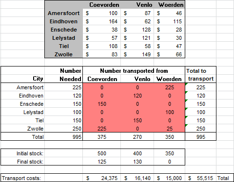
Exercise 15.8 Minimizing Transport Costs (solv008)
File: Solv008.xlsx
A company has stores in 6 cities (Amersfoort, Eindhoven, Enschede, Lelystad, Tiel, Zwolle). Stores are supplied from 3 distribution centers (DCs) in Coevorden, Venlo, and Woerden. Each week, stores forecast sales for the next week and submit the required number of products to the head office. The head office creates a transport plan based on available stock in the DCs and the required product numbers.
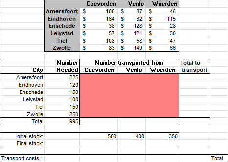
Explanation:
- The upper table shows the transport costs per product unit from a DC to a store. For example, transporting 1 product from DC Coevorden to the store in Amersfoort costs $100.
- The “Number Needed” column indicates the number of products each store requires. Amersfoort needs 225 products.
- The “Number transported from” area (the main grid in the lower section) should display the number of products transported from each DC to each store. Solver should determine these numbers.
- The “Initial stock” row contains the number of products available at each DC.
Create the cheapest transport plan using Solver.
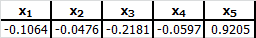
Exercise 15.9 Solving a System of Linear Equations (solv009)
Solve the following system of equations using Solver:
\[\begin{align*} 6,1x_1 + 4,5x_2 + 5,7x_4 + 7,5x_5 &= 5,7\\ 2,4x_1 + 5,5x_2 - 5,7x_3 + 4,7x_4 + 5,6x_5 &= 5,6\\ 2,4x_1 - 5,0x_2 - 4,6x_3 + 3,6x_4 + 9,7x_5 &= 9,7\\ 4,3x_1 - 5,3x_2 + 3,4x_3 - 8,4x_4 - 5,6x_5 &= -5,6\\ 1,1x_1 - 3,0x_2 + 2,4x_3 - 13x_4 + 3,5x_5 &= 3,5 \end{align*}\]
Exercise 15.10 Savings Bank Investment Strategy (solv010)
A savings bank has 3 million euros to invest. The investment portfolios include personal loans, mortgages (first and second), and car leasing. The bank association’s articles stipulate certain conditions for fund allocation:
- At least 30% of the total loaned amount must be invested in mortgages.
- At least 50% of the amount designated for mortgages must be invested in first mortgages.
- No more than 25% of the total loaned amount can be allocated to personal loans and car leasing combined.
- No more than 15% of the total loaned amount can be invested in personal loans.
The annual yield for each loan type is listed below:
| Loan Type | Yield |
|---|---|
| Personal loan | 18% |
| First mortgage | 12% |
| Second mortgage | 14% |
| Car leasing | 16% |
Determine, using Solver, how much money (in multiples of €1,000) should be invested in each of the four loan types to maximize the total annual yield.
| Loan type | Amount |
|---|---|
| Personal loan | 450 K€ |
| First mortgage | 1125 K€ |
| Second mortgage | 1125 K€ |
| Car leasing | 300 K€ |
Total yield of 422 K€. Minor differences may occur due to rounding.