7 Tables
- Characteristics of tables (lists).
- Form button.
- Merge (consolidate) data.
- Convert a data range to a table.
- Sort and filter tables.
- Calculated columns in a table.
- Column totals for a table.
Much of the information in Excel is stored in data tables, which function as a sort of database within a worksheet. While Excel isn’t a dedicated database program like MS Access, it can handle simple databases. These databases typically consist of a single table, such as address or phone lists. The term “database” is generally reserved for external files from specialized database applications. In Excel, a data table was previously referred to as a “list.”
Working with well-structured tables is common, especially in data analysis. A structured Excel table also provides an excellent foundation for creating pivot tables.
7.1 Characteristics of Tables
A table is an organized set of data.
| customnr | name | date | price | discount |
|---|---|---|---|---|
| A104 | Anderson | 2010-10-02 | 400 | 0 % |
| K102 | King | 2010-11-03 | 395 | 5 % |
| S501 | Smith | 2010-12-04 | 375 | 8% |
A table or database in Excel is composed of rows and columns. These rows are often called records, and the columns are called fields. The column contains a specific type of data. The first row of a table contains column headers that describe the information in each column. Column headers are also known as field names. The field names in Table 7.1 are: customnr, name, date, price, and discount.
For effective data analysis, it’s crucial that the data is well-structured within the worksheet. A structured table has the following characteristics:
Each column contains the same type of data.
Each row contains the individual data for a single entity or item.
The first row of the table contains unique field names. These names are usually formatted differently (e.g., larger font size, bold, italic) from the rest of the table.
The table should not contain any blank rows. A row can have empty cells, but not all cells in a row can be empty.
The table should not contain any blank columns. A column can have empty cells, but not all cells in a column can be empty.
A table can be located anywhere in the worksheet; it doesn’t have to start in the first row.
In Excel, a table is a rectangular range of cells used to store data. While a table looks similar to a regular Excel range, it offers features that distinguish it.
You can create and maintain a table by simply entering data into the cells. However, for better structure, it’s recommended to use a form for data entry. You don’t need to enter all your data before converting a range to a table; you can add new rows and columns later. Large datasets often originate from external files (text/csv files, web queries, databases).
In Excel, you can’t create an empty table and then populate it with data. Instead, you must first create a range that includes at least some of the data and then convert that range into a table. Converting a data range to a table changes its appearance and enables built-in features for filtering, sorting, and adding a total row with various aggregation functions.
By default, Excel tables automatically expand and fill formulas down to the last row. For example:
If you add new data in the row directly below the last row of the table, or in the column immediately to its right, the table will automatically expand to include the new data.
When you enter a formula in the first cell of a new blank column and press Enter, the formula automatically fills down to all the remaining rows in that column.
7.2 Form Button
Accurate data entry is essential when working with tables. Excel provides a built-in form for this purpose. However, the command button for this form isn’t on the ribbon by default. The following steps explain how to add the Form button to the Quick Access Toolbar. This is a one-time setup.
Task 7.1
- Click the Customize Quick Access Toolbar arrow at the end of the Quick Access Toolbar.
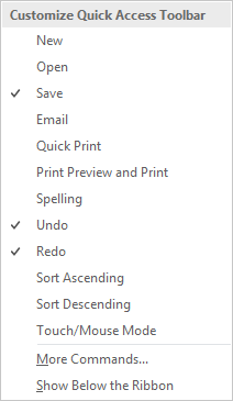
Select More Commands ….
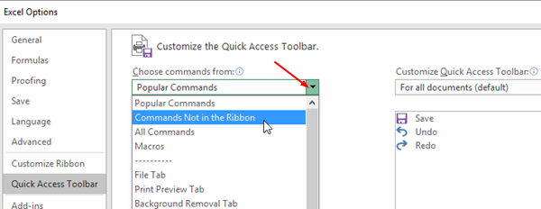
In the Choose commands from dropdown menu, select Commands Not in the Ribbon.
- Scroll through the alphabetical list of commands and select Form….
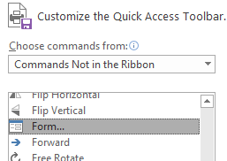
- Click Add and then click OK.
The Form button is now visible on the Quick Access Toolbar.

7.3 Data Entry Form
To complete this task, the Form button must be available on the Quick Access Toolbar (see Figure 7.4). If the button is not visible, follow the steps in Task 7.1 to enable it.
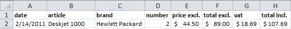
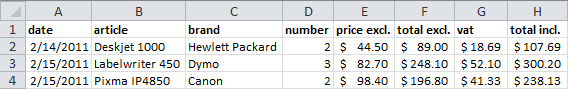
Using a data entry form is the easiest and most effective way to add records to a table. Excel can automatically generate a form if you provide the column field names and enter the first record. The following figure shows an example of a purchase list. The data for the first item, including the formulas in cells F2, G2, and H2, has already been entered.
Task 7.2 File: Purchases.xlsx
Open the file.
Enter the following formulas:
- F2:
=D2*E2 - G2:
=21%*F2 - H2:
=F2+G2
- F2:
Select any cell within the list.
Click on the Form button on Quick Access Toolbar.
The data form appears, displaying the eight field names on the left. Entry boxes are provided for five of the field names, allowing you to enter or modify data. The fields total excl., vat, and total incl. display values because they are calculated using formulas.
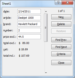
- Click New and add two new records (see the example in Figure 7.7). Click Close after entering the last record.
Use the Tab key or the mouse to navigate between fields. Pressing the Enter key moves you to the next record, or creates an empty form for adding a new record if there are no more records.
7.4 Searching Data with a Form
A data form is also useful for searching a range or table for records that meet specific criteria. The following task demonstrates this. Examples of how to apply criteria are provided at the end of the task.
Task 7.3 File: Personnel.xlsx
Open the file.
Select any cell in the data area.
Click the Form button. The data form appears.
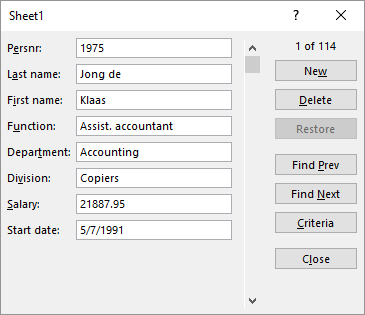
Click Criteria. The form clears and is ready for you to enter search criteria.
Search for the “Accounting” department and the “Printers” division (see Figure 7.9).
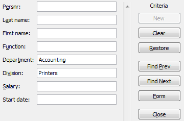
Click Find Next. The data of the first person matching the criteria is displayed.
Use the Find Next and Find Prev buttons to browse through the list. There are five people who meet the criteria.
7.4.0.1 Examples of Search Criteria
Table 7.2 provides examples of search criteria. Try these examples to confirm that the found records match the criteria. You can also combine multiple criteria. Remember to clear the criteria list before starting a new exercise.
| Field | Value | Explanation |
|---|---|---|
| Last name | Ja | Searches for people whose last name starts with “Ja”. |
| Last name | *os | Searches for people with “os” in their last name. |
| Salary | >70000 | Searches for people with a salary greater than 70000 |
| Start date | <1/1/1990 | Searches for people with a start date before 1/1/1990 |
7.5 Consolidating ranges
You can summarize (consolidate) similar data from different ranges into a new range. In practice, the source ranges are often in separate worksheets, and the consolidated range is placed in a new worksheet.
When you consolidate source data, you apply a summary function (SUM, AVERAGE, COUNT, etc.) to create the summary data. The columns must have a heading or label to consolidate ranges.
Task 7.4 File: Consolidation.xlsx
Open the file.
Select cell A1 in the “Total” worksheet.
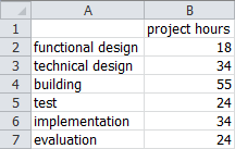
The lists to be summarized are in the “PRA” and “PRB” worksheets. The consolidated data will be placed in the “Total” worksheet.
- Go to Data > Consolidate (Data Tools group).
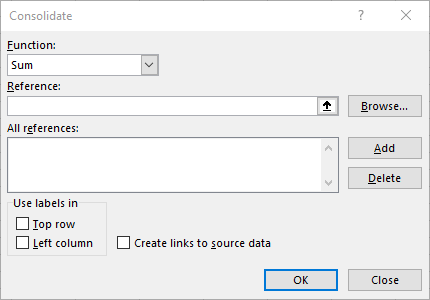
Ensure that the
SUMfunction is selected. If not, select it.Click in the Reference box.
Select worksheet PRA > range A1:B7 > Add and click Add.
Select worksheet PRB > range A1:B7 > Add and click Add.
Check the Top row and Left column boxes under “Use labels in.”
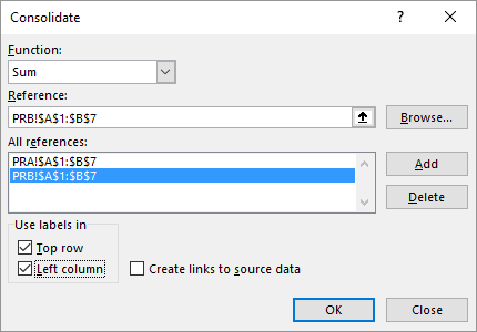
- Click OK.
Consolidation is static. If the source data changes, the consolidation results will not update automatically. You’ll need to perform a new consolidation. Using pivot tables is often a better approach for summarizing data.
7.6 Convert Range to Table
Converting a range or list to an Excel table unlocks the additional features and capabilities of tables.
Task 7.5 File: Candyboxes.xlsx
Open the file and select any cell within the data range.
Go to tab Insert > Table
The Create Table dialog box appears. If you previously selected a cell with data, the range to be converted is automatically filled in. If not, or if the range is incorrect, select the correct data range, including the headers.
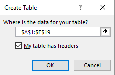
If your range includes labels that you want to use as column headers, check “My table has headers.” If there are no labels, uncheck this option. Excel will automatically add headers with generic names: Column1, Column2, etc.
It’s strongly recommended that you provide your own descriptive headers.
- Click OK.
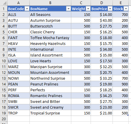
After converting a range to a table, you’ll notice the following changes:
A table format (style) is applied. You can change this to a different format if desired.
Each column header now has dropdown arrows for filtering and sorting.
A Table Design tab is added to the ribbon. This tab is only visible when a cell within the table is selected.
7.6.1 Table Design
The Table Design tab allows you to manage various table settings.
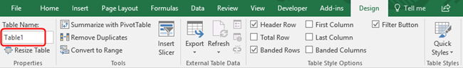
Each table is automatically assigned a Table Name. The default names are Table1, Table2, Table3, etc. It’s best practice to change the default name to a meaningful name that reflects the table’s data. This name is used when referencing the table and in table operations.
You can change the name in the Table name box.
7.7 Table Operations
7.7.1 Selecting Rows/Columns in a Table
Right-click a cell in the row or column you want to select.
Choose Select, and then select one of the following options:
- Table Column Data
- Entire Table Column
- Table Row
7.7.2 Inserting a Table Row/Column
Right-click a cell.
Choose Insert and then select one of the options:
- Table Columns to the Left
- Table Rows Above
If you select a cell in the last row or last column, you’ll also have the options:
- Table Column to the Right
- Table Row Below
If you select the last cell (bottom right), you’ll have both options.
A quick way to add a new row is to select the bottom-right cell and press the Tab key.
7.7.3 Deleting a Table Row/Column
Right-click a cell in the row or column you want to delete.
Choose Delete, and then select one of the options:
- Table Columns
- Table Rows
7.7.4 Convert a Table to a Range
Select any cell inside the table.
Go to tab Design (Table Tools) > Convert to Range ( Tools group) and confirm the operation.
7.7.5 Apply a Table Style
Select any cell inside the table.
Go to tab Design.
Choose a style from the Table Styles gallery.
7.8 Sort a Table
Sorting is a common operation with lists. If you select a cell in a column and click the sort button, the entire table will be sorted. It can be sorted in ascending or descending order based on the values in that column.
The only way to restore the table to its original order is by using the Undo button on the Quick Access Toolbar. Alternatively, before sorting, you can insert a temporary column with sequential numbers. Sorting by this column later will return the table to its original state.
Task 7.6 File: Personnel.xlsx
Open the file.
Convert the data range to a table (see Section 7.6).
Click the arrow next to the Department field name and select
 Sort A to Z.
The table is sorted in ascending order of the column Department.
- Click on the arrow next to the Division field name and select
 Sort Z to A .
The table is sorted in descending order of the column Division.
You can sort a table on multiple levels, based on the values in different columns. One of the columns will be the first level where you sort on. After that, you can add new levels of sorting. Another column provides the second level of sorting, etc.
- Select any cell in the table and go to Home > Sort & Filter (Editing group) > Custom Sort ….
The Sort dialog box appears, where you can specify the sort conditions.
Choose to sort by Division.
Click Add Level and then choose to sort on Department.
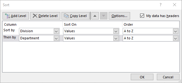
- Click OK.
First, the values in the column Division are sorted in ascending order, and then the values in the Department column are sorted..
7.9 Filter a Table
When you filter a table, only the records that meet specific conditions are displayed. The other records are hidden.
Task 7.7 File: Personnel.xlsx
Open the file.
If it isn’t already, convert the data range to a table (see Section 7.6).
Click the arrow next to the Division field name, select only “Copiers,” and then click OK.
Only the records for the Copiers division are now displayed. The arrow in the Division column header changes to the filter symbol ![]()
- Now, refine your selection by filtering for the Accounting department.
The status bar at the bottom displays the number of records found.
- Clear the filter by going to Data > Clear (Sort & Filter group).
7.9.1 Number Filter
When a field contains numbers, you can use specific filter actions. These filters are in the Number Filters category. The following example demonstrates how to find the top 10 salaries.
Task 7.8
- Click the arrow next to the Salary field name and select Number Filters > Top 10….
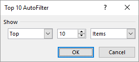
You can change 10 to a different number. You can also change Top to Bottom.
Click OK. The 10 records with the highest salaries are now displayed.
Clear the filter by going to Data > Clear (Sort & Filter group).
7.9.2 Custom Filter
For number field filters other than the default filters, use a custom filter. The following example shows how to display records for people with salaries from $20,000 to $25,000.
Task 7.9
- Click the arrow next to the Salary field name and select Number Filters > Custom Filter….
The Custom AutoFilter dialog box allows you to specify filter conditions.
- Create the two salary conditions as shown in Figure 7.18.
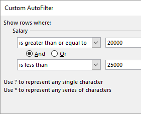
Click OK. 10 records are found.
Clear the filter by going to Data > Clear (Sort & Filter group).
7.9.3 Date Filter
When a field contains dates, you can use specific filter actions for dates. These filters are in the Date Filters category. The following example shows how to find records with a start date in September.
Task 7.10
Click the arrow next to the Start date field name and select Date Filters > All Dates in the Period > September.
11 records are found.Clear the filter by going to Data > Clear (Sort & Filter group).
7.9.4 Slicers
A slicer is an Excel object that you can use to filter data. It displays all the unique values from a selected column, with each value as a button. Slicers are faster to use than traditional filters, and they provide immediate visual feedback on what is being filtered.
Slicers can be used with both tables and pivot tables (see Section 13.5.2). They appear to float above the spreadsheet, making them readily accessible.
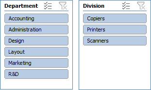
Task 7.11
Select any cell in the table.
Go to tab Table Design > Insert Slicer (Tools group).
The Insert Slicer dialog box opens and displays the column headings (fields) for which you can insert a slicer. You can select one or more fields.
- Select the Department and Division fields and click OK.
Two slicers are inserted. If they overlap, move them so that they are next to each other, as shown in Figure 7.19. Both slicers display all the unique values for their respective fields.
In the Department slicer, click the Marketing button. Only the data for Marketing is now displayed.
Clear the filter by clicking the Clear Filter button (the button with the “x”) in the top right corner of the Department slicer.
In the top right corner of the Department slicer, click the Multi-Select button. Now, filter for both Administration and Marketing.
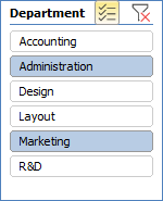
The buttons act like toggles. Clicking a button repeatedly turns the filtering for that value on and off.
Now, select Printers in the Division slicer.
Experiment with the slicers. You can optionally add a third slicer for the Function column. When you’re finished, clear all filters.
7.10 Calculated Column
When you enter a formula into an empty table column, that formula automatically extends to the rest of the column. You don’t need to use Fill or Copy. This type of column is called a calculated column. If you change a formula, the change automatically applies to the entire calculated column.
The easiest way to create a new calculated column is to start typing in the column immediately to the right of the table. The table will automatically expand to include the new column.
Task 7.12 File: Personnel.xlsx
Open the file.
If it isn’t already, convert the data range to a table (see Section 7.6).
Select cell I2 and enter the formula
=ROUND([@Salary],0). A new table column with the calculated values is created.
References like [@Salary] are called structured references, which are unique to Excel tables. Structured references allow the table to use the same formula for each row.
Change the column header to
Rounded Salary.Select a numeric cell in the new column, then Right-click > Select > Table Column Data.
Change the cell format to
Accounting, 0 decimals.Select cell J2 and enter the formula
=YEAR(NOW())-YEAR([@[Start date]]).Change the column header in
Age.
7.11 Task: Total Row
You can summarize numeric data in a table using a subtotal that appears at the bottom of the table. Although the term “subtotal” suggests summing numeric values, Excel uses it more broadly. A subtotal can be a sum, average, maximum, minimum, standard deviation, variance, or count of the values in a field. The calculation is based on the visible cells in the table’s column.
Task 7.13 File: Personnel.xlsx
Open the file.
If it isn’t already, convert the data range to a table (see Section 7.6).
Go to Table Design tab> Check the Total Row box (Table Style Options group)
A “Total” row is inserted at the bottom of the table, and a SUBTOTAL function is added below the last column. In this case, the function is irrelevant because the last column is a date column.
In the “Total” row, select the cell below the Start date column, click the dropdown arrow
 and choose “None”.
In the “Total” row, select the cell below the Salary column, click the dropdown arrow
and choose “Sum”.
The total salary is $ 4,874,037.39.
7.12 Exercises
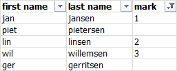
Exercise 7.1 Filtering (list001)
File: List001.xlsx
The following table lists the grades of some students.
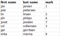
Apply a filter to display only the rows for students with no grade or a grade of 3 or lower. This exercise uses a small table. Your solution should work for much larger tables.
Exercise 7.2 Consolidating Examination Results (list002)
File: List002.xlsx
The following table shows the results of a group of students for an examination and a re-examination. It also shows the final result, which is the highest grade.
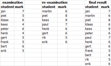
Enter the examination and re-examination data in a worksheet. Determine the final result using consolidation.
Exercise 7.3 Consolidating Sales Data (list003)
File: List003.xlsx
The following table lists the sales numbers of bread types in the North and South branches of a store. It also shows the total sales numbers obtained by consolidation.
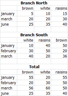
Enter the data for the two branches in a worksheet. Determine the totals using consolidation.
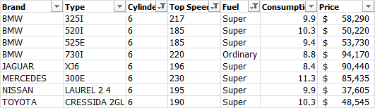
Exercise 7.4 Filtering Car Data (list004)
File: Car.xlsx
In a worksheet, you can find some data of cars. A customer is interested in cars that meet the following conditions:
- 6 cylinders
- Top speed of at least 180 km/hour
- Petrol (regular or premium) fuel type
Create a list of all cars with their data that meet these conditions.