4 Formatting worksheet and data
Excel offers many opportunities for the appearance of a worksheet and data in cells. This can make a worksheet more readable and presentable.
You can apply a format (for example the font type) to the entire worksheet, or individual cells or areas of cells. The process is usually the same, but it depends on what is selected.
First select, then execute the format command.
You can select the entire worksheet through the button to the left of the first column and above the first row: 
4.1 Column Width
A column could be too small to display the entire contents of a cell. If the content of the cell is a text, you will see only that part of the text that fits into the cell. If the content of the cell is a number, you will see “hashes”: ####.
In a worksheet, you can specify the column width from 0 (zero) to 255. This value represents the number of characters that can be displayed in a cell that is formatted with the default font. The default width of columns in Excel is 8.43. Eight characters with the default font fit then in a column. If the width of a column is 0, then the column is hidden.
There are several ways to adjust the width of a column.
Double-click the right edge of the column heading. The width of the column is now automatically set to the longest text in the column.
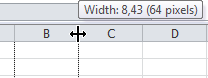
Place the mouse pointer over the right edge of the column header, press the left mouse button, and drag the right edge of the column to the left or to the right until the column has the desired width. While dragging Excel displays the current width of the column in a small information screen.
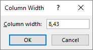
Adjusting column width through dragging Right-click the column header and select Column Width from the shortcut menu. In the dialog box, you can enter the desired width of the column, after that click OK.
Specifying column width Select a cell in the column of which the width must be adjusted. Then choose Home > Format (group Cells) > Column Width…. You’ll get the same dialog as before.
You can adjust the width of multiple columns simultaneously. First, select these columns using the SHIFT-key or CTRL-key .
You can change the width of all columns in the worksheet through Home > Format (group Cells) > Default Width...
4.2 Row Height
Normally, row heights will change automatically to accommodate the size of the data in the row. But for formatting purposes, it is sometimes necessary to adjust the height of a row. You can specify the height of a row from 0 (zero) to 409. This value represents the height in points (1 point is about 0.035 cm). The default height of rows is 12.75 points (about 0.4 cm). When the row height is 0, the row will be hidden.
There are several ways to adjust the height of rows.
Double-click the boundary below the row heading. The height of the row will auto-fit the contents of the row.
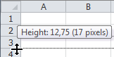
Place the mouse pointer over the right edge of the row heading, press the left mouse button and drag the border of the column up or down until the row has the desired height. While dragging, Excel displays the current height of the row in a small information screen.
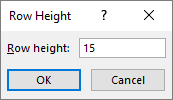
Adjusting row height through dragging Right-click the row heading and select Row Height… from the shortcut menu. In the dialog box, you can enter the desired height of the row, after that click OK.
Specifying row height Select a cell in the column whose width must be adjusted. Then choose Home > Format (group Cells) > Row Height…. You’ll get the same dialog as before.
You can adjust the height of multiple rows simultaneously. First, select these rows using the SHIFT-key or CTRL-key .
4.3 Font
The group Font (tab Home) has several commands that allows changing the appearance of text in cells. To apply these changes, you must first select the cell(s) and then use the command button. The options in this group are:
 : Font, choice list through the down arrow.
 : Font size, choice list through the down arrow.
 : Increase / Decrease Font size, always in steps of 2 points.
 : Style, successively: bold, italic, underlined. The specific underscore can be determined using the down arrow.
 : Font color, the color can be chosen through the down arrow.
 : Fill color, the color can be chosen through the down arrow.
4.4 Cell Borders
Borders are often used to hold a group of cells visual together. Under an addition, there is often a line and below the line - the total. Borders are used especially for layout purposes.
To create borders around a cell or group of cells, proceed as follows:
Select the cell or the group of cells.
Choose Home > Border down arrow (group Font).

Choose the desired style from the list Borders.
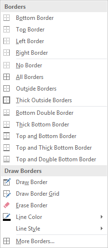
If the desired border style is not displayed in the list, then click on More Borders…. Excel displays the dialog box Format Cells with the tab Border selected.
4.5 Cell Alignment
How to align the content in cells, horizontally, vertically, and even rotated.
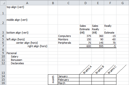
A cell has a vertical and horizontal alignment. By default, the vertical alignment is the bottom alignment for all cells. The default horizontal alignment is left-align for text, right-align for numbers and center-align for logical values (TRUE or FALSE ). You can change all these alignments as you can see in Figure 4.2.
To apply a particular alignment, first select the cell(s) and then click one of the buttons in the group Home > group Alignment.
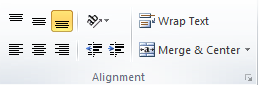
The buttons don’t need an explanation. When you hover the mouse over a button you get some explanation.
In the example, the following options are used.
- Vertical alignment
-
The options are top, middle, bottom. Applied in the cells A1:A3.
- Horizontal alignment
-
The options are left, center, right. Applied in the cells A5:A7.
- Indentation
-
The options are increase indent, decrease indent. Applied in the cells A10:A12.
- Orientation
-
With this button, you get some predefined options. Applied in the cells D13:F13 and in B14.
- Wrap Text
-
The text appears on multiple lines in the cell. For this, the row height will be made larger. A long text will take less horizontal space. Applied in D3:F3.
If all wrapped text is not visible, the reason could be that the row is set to a specific height. To allow the row to adjust automatically and show all wrapped text, choose Home > Format (group Cells) > AutoFit Row Height.
- Merge & Center
-
Joins the cells into one larger cell and centers the content in the new cell. This is often used to create labels that span multiple rows or columns. You can join cells both horizontally and vertically. Applied in B14:B16.
4.6 Formatting Numbers
Numbers can be displayed in different ways, with or without decimal places, with a currency symbol, with various separators for date or time, etc. And if the predefined formatting options are not enough, you define your custom format.
When entering some numbers, Excel puts them in the correct format automatically.
If you enter
19%in a cell, then Excel will recognize the percent symbol and displayed the number right-aligned as 19%. The content of the cell will be 0.19 and not 19.If you enter
€123,45in a cell, then Excel recognizes it as a currency. The content of the cell will be 123,45 and this content will be displayed right aligned as € 123,45.If you enter
1/2in a cell, then Excel thinks that it is a date and displayed it as 2-Jan.
Excel stores dates and times as serial numbers starting with 1 January 1900 as number 1. Number 2 is then 2 January 1900, etc. And if you enter 1/2 in a cell, then the current year will automatically be added, for example, 1/2/2013 and then the real content of the cell will be 41276.
To quickly assign a format to a number, use of the command buttons in the Number group (tab Home).
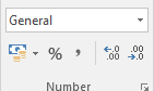
In the middle you find command buttons for some frequently used formatting styles:
 : Accounting style. The down arrow gives some currency symbols.
 : Percent style.
 : Comma style (thousands separator)
 : Increase decimals.
 : Decrease decimals.
At the top, you can see the actual formatting of the selected cell. For example General and beside a down arrow for a choice list with predefined styles. In the figure, you can see this list for a cell with content 0.19. And in this list, you can choose another format.
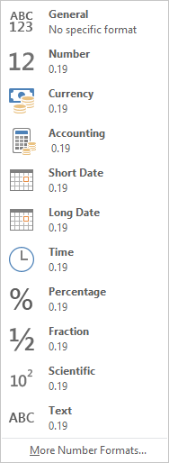
When the desired formatting is not on the list then you can click on More Number Formats…. The dialog box Format Cells appear with the tab Number selected. Here you can define your custom format.
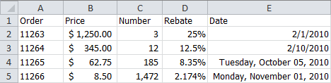
In the following example, you see a part of a worksheet containing many uses of number format. All formatting has been applied with the predefined styles and / or the command buttons for number formatting.
Task 4.1 File: Numberformat.xlsx
Open the file.
Format the worksheet as shown in the figure. Use of the opportunities available through the group Number (tab Home).
- Column A, numbers formatted as text.
- Column B, accounting number format.
- Column C, numbers formatted first with the thousands separator and then decreased the number of decimals to 0.
- Column D, numbers entered with the percent symbol and then adjust the number of decimals.
- Column E, dates entered, applied the short date format for the first two, and the long date format for the last two.
4.7 Copying and clearing format
The format and content of a cell are stored separately. Therefore, you can separately copy or delete the content and format.
Copying format
The fastest way to copy the format of a cell to another cell is to use the button Format painter.
The method is as follows:
- Select the cell with the format you want to copy.
- Choose Home >
 (group Clipboard). The mouse shape changes in a brush (
 ).
). - Select the cell(s) you want to transfer the format to.
- Release the mouse button.
When you double click on the button Format painter then you can perform multiple format transfers. To cancel format copying you can click again on the button Format painter or press the Esc key
Removing format
The format of cells can be removed as follows:
Select the cell(s) which format you want to remove.
Choose Home > Clear (group Editing) > Clear Formats.
This way you can clear the format, the content, or both.
With the DELETE key you only clear the content of the cell. The format of the cell (font type, colors, alignment, number format, etc.) will not be changed and is still present in the empty cell.
4.8 Table Styles
To practice the formatting of a list with one of the predefined styles.
Excel has several predefined styles for formatting a list (table) quickly and easily.
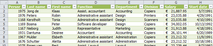
Task 4.2 File: Personnel.xlsx
Open the file.
Select any cell in the data area.
Choose Home > Format as Table (group Styles).
Choose a style from the examples shown, for example, Table Style Medium 4.
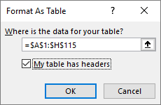
- Click OK.
4.9 Conditional Format
The format of a cell can depend on certain conditions. For example, the background of the cell can be made red when the value in the cell is less than 6. This is called a conditional format. The formatting is applied if the condition(s) are met. If not, the “ordinary” format will be applied.
To apply conditional formatting, you can use any combination of the following formatting options: number format, font, border, and background.
In the condition test, the numerical value in the cell(s) will be compared with a different value. You can also compare the numerical value with a range of other values to determine whether there is a deviation from the average or, for example, belongs to the top three. There is no limit to the number of conditions.
4.9.1 Format with 1 condition
A teacher has the marks of his students in a spreadsheet and wants to provide all failures (marks less than 6) of a light red background.
Task 4.3 File: Marks.xlsx
Open the file.
Select all marks.
Choose Home > Conditional Formatting (group Styles) > Highlight Cells Rules > Less Than… and enter in the dialog box the desired condition and format.
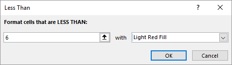
- Click OK. All failures have a light red background color now.
Test the conditional format by changing the values in some cells from insufficient to sufficient and vice versa. The background color has to change now.
4.9.2 Format with 2 conditions
In a spreadsheet, the realized turnover and the turnover to be achieved of the salesmen are tracked. Some of them have not met their target. The task is to apply the background for the turnover with one of the following colors: green if the target has been met and red if the target has not been met.
Task 4.4 File: Turnover-Q1.xlsx
Open the file.
Select all cells with the turnover data.
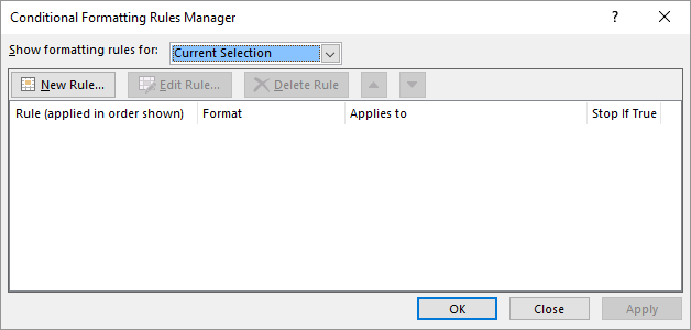
Choose Home > Conditional Formatting (Group Styles) > Manage Rules….
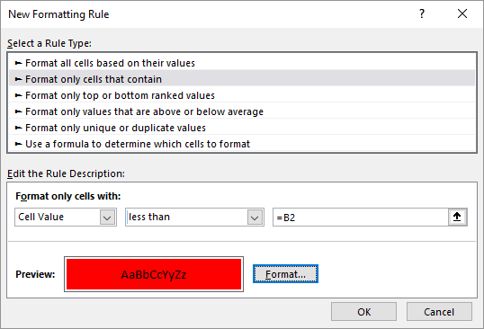
Click on New Rule…. The dialog box New Formatting Rule appears.
Select Format only cells that contain, then specify Cell Value less than
=B2and choose a red fill color as Format.
Click OK. The dialog box Conditional Formatting Rules Manager appears again.
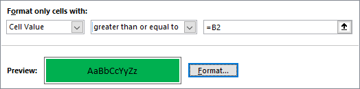
Click on New Rule and create a new rule on the same way with the following settings:
- Click OK. In the manager screen now there are two rules:
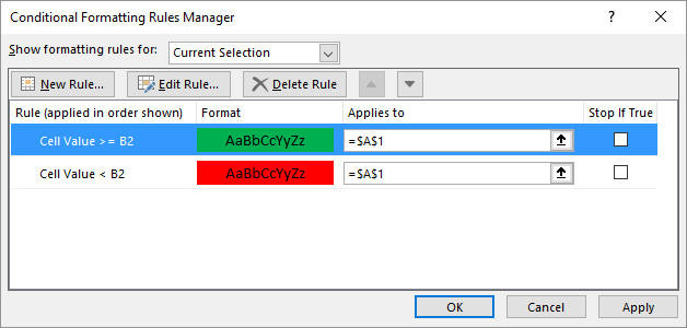
- Click OK. The desired format will be applied now.
Test the conditional format by changing some values and make sure that the format will change.
4.9.3 Format for top/bottom 10%
It is possible to create a condition that depends on all values in a set. For example, you can create a conditional format for the top/bottom three in a set of values, or the worst or best 10% values.
In a spreadsheet are all kinds of data from cars. In one of the columns, you can find fuel consumption. The task is to give a green background color to the 10% cars with the lowest fuel consumption.
Task 4.5 File: Car.xlsx
Open the file.
Select all consumption values in column F.
Choose tab Home > Conditional Formatting (group Styles) > Top/Bottom Rules > Bottom 10%… and enter the desired values in the dialog box.
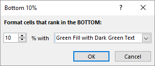
- Click OK.
4.9.4 Removing conditional formats
A conditional format can be removed as follows:
Select the cell(s) with the conditional format.
Choose tab Home > Conditional Formatting (group Styles) > Clear Rules > Clear Rules from Selected Cells.
4.9.5 Finding conditional formats
Sometimes it is difficult to see if there are cells in a worksheet with conditional formatting. Excel provides support to find them. This is done as follows:
Choose tab Home > Find & Select (group Editing) > Conditional Formatting.
All cells with a conditional format are now selected. If there are no cells with a conditional format, Excel displays the following message: No cells were found.