12 Data Tables
A data table is a tool for “What-if” analyses. For formulas with 1 or 2 variables, you can quickly calculate the results for different values of the variables. So you can track how small changes in input values affect the results of formulas that are dependent on those input values. For example, how changes in the price of an article affect the sales of the company. An analysis of this sort is often termed a sensitivity analysis. The only limitation is that you can use a maximum of two variables in the formulas.
Excel has two varieties of data tables:
- One-variable data table, working with one input variable and one or more formulas.
- Two-variable data table, working with two input variables and one formula.
Both types of data tables work the same way:
- Define a set of input values for the variables.
- Identify the formulas dependent of these variables.
- Execute the Data Table command.
Then Excel substitutes each one of the input values in the formulas, calculate the results, and shows these in a table form.
12.1 One-variable Data Table
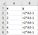
If you want to calculate the result of a formula with one variable for different values of that variable, you can do that by creating two columns, one with values for the variable and the other with the outcomes of the formula.
Figure 12.1 shows this for the formula \(y = 2*x - 1\).
In those cases, it is much more convenient to create a data table with 1 input cell.
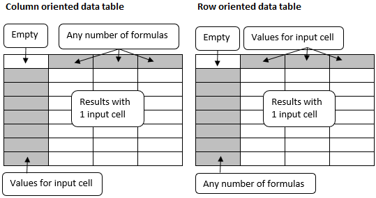
In a column orientated table are your variable values in a column and the formula one row above and one cell to the right of the column of the values. You can type additional formulas in the cells right of the first formula.
If the data table is row-oriented then your variable values are in a row and the formula(s) in the cell one column to the left of the first value and one cell below the row of values. You can type additional formulas in the cells below the first formula.
The input cell can be any cell on the worksheet. Excel uses this as a temporary repository. The formulas must have a reference to this input cell. The values for the variable are sent to this input cell, then the result is calculated and placed in the table.
Instead of formulas you can also use references to formulas.
12.2 Rental cottage
A simple example of a data table with 1 input cell.
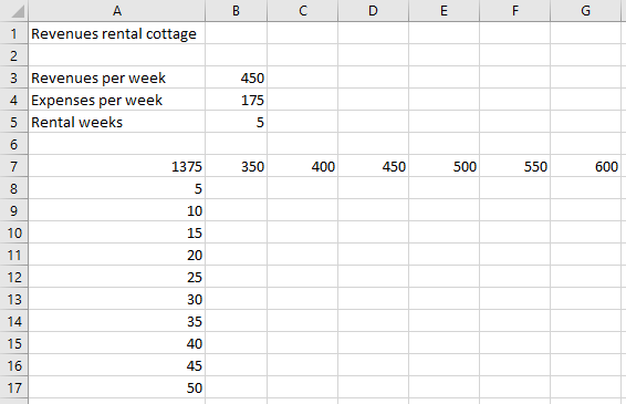
A summer cottage can be rented for 450 dollars a week. The expenses per week are 175 dollars. Using a data table, calculate the revenues for 5, 10, 15, …, 50 weeks.
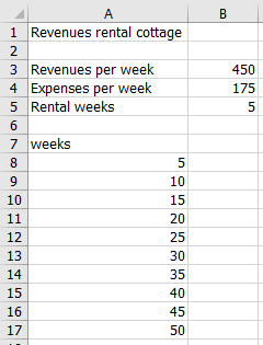
The data table will be in A7:B17. The formula with a reference to the input cell B5 comes in B7. The values for the variable are in range A8:A17 and the results are going to B8:B17.
Task 12.1 File: Rental_fixed.xlsx
Open the file.
Type in cell B7 the formula
=B5*(B3-B4).Select the range for the data table A7:B17.
Choose tab Data > What-If Analysis (group Forecast) > Data Table.
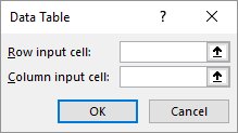
- Put the cursor in the box Column input cell and click then on cell B5.
Excel transforms the cell address to $B$5.
- Click OK.
The data table will be filled with the calculated values.
The formula in the result cells is an array formula: {=TABLE(,B5)}. Check this.
12.3 Calculating multiple values of formulas
An example using a data table with 1 input cell to calculate the values for multiple formulas.
The task is to calculate the y-values of four functions for different x-values.
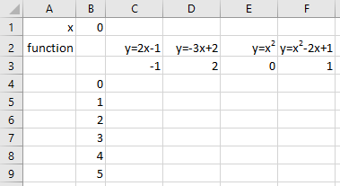
The input cell will be B1. This is the cell where the different x-values are added. What formulas are used can be seen in the cells C2:F2. The formulas themselves are in the cells C3:F3. The x-values are in the cells B4:B9.
Task 12.2 File: Function_values.xlsx
Open the file.
Add the correct formulas in cells C3:F3:
- C3:
=2*B1-1 - D3:
=-3*B1+2 - E3:
=B1^2 - F3:
=B1^2-2*B1+1
- C3:
Select the range for the data table B3:F9.
Choose tab Data > What-If Analysis (group Forecast) > Data Table.
Put the cursor in the box [Column input cell] and then click on cell B1.
Click OK.
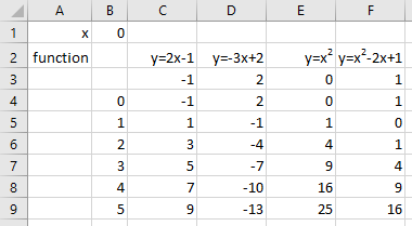
The formula in the result cells is an array formula: {=TABLE(,B1)}. Check this.
12.4 Two-variable Data Table
The two-variable data table uses a formula that contains two lists of input values. The formula must refer to two different input cells: the row input cell and the column input cell.
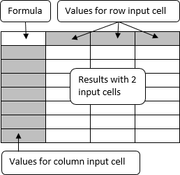
The overall layout looks like a data table with 1 input cell, but there are some important differences:
- A data table with 1 input cell can evaluate multiple formulas, while with 2 input cells only the results from 1 formula can be calculated.
- The values for the variables are both in a column and a row.
- The upper left cell must contain the formula (or a reference to the formula).
12.5 Rental cottage with variable price
An example of a data table with 2 input cells
A summer cottage can be rented for 350-600 dollars a week, the price depends on the season. The expenses are fixed on 175 dollars per week. Using a data table, calculate the revenues for 5, 10, 15, …, 50 weeks and rental prices 350, 400, 450, … 600.
The data table will be in A7:G17. The two input cells are B3 (rental price) and B5 (number of rental weeks). In cell A7 is a formula with references to the two input cells. The values for input cell B3 are in row B7:G7. The values for input cell B5 are in column A8:A17.
Task 12.3 File: Rental_variable.xlsx
Open the file.
Enter in cell A7 the formula
=B5*(B3-B4).Select the range for the data table A7:G17.
Choose tab Data > What-If Analysis (group Forecast) > Data Table.
Put the cursor in the box Row input cell and click on cell B3.
Put the cursor in box Column input cell and click on cell B5.
Click OK.
The formula in the result cells is an array formula: {=TABLE(B3,B5)}. Check this.
12.6 Revenues advertising campaign
An example of a data table with 2 input cells for the calculation of the effect of an advertising campaign.
A company wants to run an advertising campaign by sending direct mail flyers to potential customers. Use a calculation model, to calculate the expected profit of this advertising campaign.
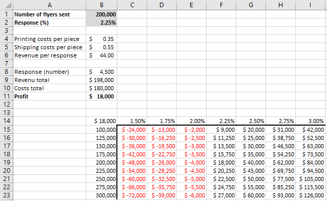
The calculation model uses 2 variables: the number of flyers sent and the response percentage. The printing and shipping costs are fixed data, as well as the expected revenue per response. The number of responses and total revenues, costs, and profits is calculated using formulas.
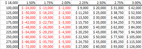
The range for the data table is B14:I23. The two input cells are B1 and B2. The values for input cell B1 are in column B15:B23. The values for input cell B2 are in row C14:I14. In cell B14 is a reference to the total profit formula, which in turn references to the two input cells.
Task 12.4 File: Advertising_Campaign.xlsx
Open the file.
Select the range for the data table B14:I23.
Choose tab Data > What-If Analysis (group Forecast) > Data Table.
Put the cursor in the box Row input cell and click on cell B2.
Put the cursor in the box Column input cell and click on cell B1.
Click OK.
The formula in the result cells is an array formula: {=TABLE(B2,B1)}. Check this.
12.7 Exercises
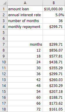
Exercise 12.1 Repayment Loan (tabl001)
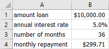
A loan of $10,000 must be repaid in some monthly periods at an annual interest of 5%. The calculation of the monthly amount to repay is calculated with the PMT function. In the following figure, you can see this for a payment period of 36 months.
- Make the above model in a new worksheet and create a formula for the monthly repayment.
- Create a data table with an overview of the monthly repayments for redemption periods of 12, 18, 24, 30, …, 72 months.
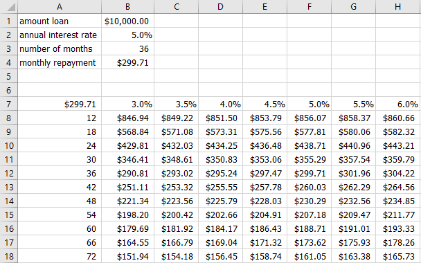
- Create a new data table with an overview of the monthly repayments for redemption periods of 12, 18, 24, 30, …, 72 months, and annual interest rates of 3%, 3½%, 4%, 4½% … 6%.
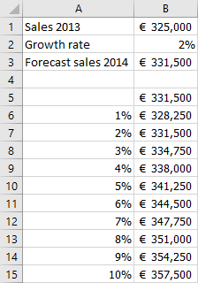
Exercise 12.2 Sales forecast (tabl002)
In a worksheet the forecast of the sales in 2014, based on the sales in 2013 and an estimated sales growth.
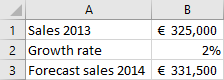
- Make the above model in a new worksheet and create a formula for the forecast of the sales in 2014.
- Create a data table with an overview of the sales forecast with growth rates of 1%, 2%, … 10%.